Everything is Significant

We’ve briefly talked about how $p$-values should be interpreted. It’s crucial to understand that a $p$-value of 0.01 doesn’t mean that there is a 1% chance of some null hypothesis being true. Instead, it implies a 1% chance of observing data as extreme or more extreme than the current data under the condition that the null hypothesis is true.

$p$-values form the foundation of frequentist statistics, and rightfully so because it determines whether a certain event (alternative hypothesis) is probably true by thresholding it against a determined significance level and repeating the experiment many times. However, it’s precisely because the $p$-value is what makes or breaks research (the woes of spending a whole year to find out a proposed hypothesis is not significant) that some unethical researchers manipulate it, a term coined $p$-hacking. Not limited to being intentional, careless practitioners can also accidentally hack these probabilities.

***

I used to go door-to-door pitching my tutoring services back in college. At the same time, I’ve always wondered if I would’ve gotten more callbacks if I had just posted my services on Facebook. This determination is called A/B testing, which serves a perfect example to showcase how p-hacking works and can be avoided.

Let’s consider the door-to-door as the control and online ads as treatment. To start off, we form our hypotheses:

• $H_0$ : Both the control and treatment methods are equally effective
• $H_1$ : The treatment is more effective than the control

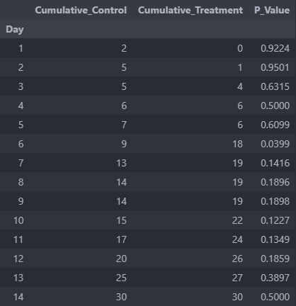
Next, we assume the proper testing methodology, that is, we lay out our plan even before starting the experiment to avoid bias. We’ll collect data in terms of number of callbacks per 100 people reached in each group for 14 days. We conclude on a hypothesis only after the experiment at a significance level $\alpha = 0.05$. After running the experiment, we obtain the following results:

Now comes the fun part where we put ourselves in the shoes of an unethical scientist. In fact, we’ll make sure to tick as many $p$-hacking boxes as we can throughout our analysis.

Early Stopping

Since we calculate the running $p$-values, having seen an outcome we like on day 6 ($p=0.040<\alpha$), we simply stop the experiment and declare posting ads on Facebook the winner. Unfortunately, we’ve just fallen into a sequential testing bias.

In statistics, setting $\alpha=0.05$ states an expression of willingness to accept a 5% risk that pure randomness could produce a result extreme enough to be mistaken for a real effect (Type I error). When we check the $p$-value multiple times as data accumulates, we’re essentially inflating the Type I error rate to

where $k$ is the number of times we peek at the data. For our case, there’s actually a 26.5% of seeing a false positive on the sixth day!

To avoid this, we should simply just let the experiment run its course and check the $p$-value at the very end, therefore keeping the Type I error rate at exactly $\alpha$. If not, we could also introduce a stricter threshold:

In this case, we see that the threshold on the sixth day ($k=6$) is actually 0.0083, which renders our $p$-value of 0.040 insignificant.

Additional Data Collection

Let’s imagine that $p>\alpha$ for day 6 instead, such that we never actually observe the $p$-value indicate significance. Since we’re desperate to want to see Facebook win, we cheekily continued the experiment another day, then another day, then another day… until we eventually observe $p<\alpha$.

This is another example of sequential testing bias. Again, by running additional experiments and peeking at the $p$-values along the way, we’re simply inflating the Type I error rate. The fix for this is exactly the same as that explained in the early stopping early section.

Data Transformation

We decided to neither stop early nor collect more data. Now, the $p$-value isn’t significant but we want it to be. So we start transforming the data in multiple ways—square-root, inverse, log. As it turns out, after a log transformation, $p$-value becomes 0.042!

Why is this wrong? Every statistical test has assumptions. Normal distribution, homoskedasticity, linearly related variables, etc. When we transform data, the assumptions for the tests may be violated, rendering the conclusions invalid. On top of that, even if we’ve made sure that the assumptions have been approximately met, the issue is, again, inflated Type I error rate. This is because by running multiple tests, we’re essentially peeking multiple $p$-values, which, as explained, increases the chances of stumbling upon a spurious significant result.

To fix this, only transform the data if there’s a legitimate statistical reasoning behind it. We shouldn’t let the outcome ($p<\alpha$) dictate which statistical assumption we adopt.

Multiple Method Testing

Okay then. If we can’t transform our data according to what we want, we’ll just evaluate the data with different statistical tests: chi-square, Fisher’s exact, Mann-Whitney U, … Bingo—Mann-Whitney U test outputs a $p$-value of 0.048.

The issue is exactly like that for data transformation. First, the tests have assumptions that may be invalid given the data. If this isn’t the case, then the problem is, again, we’re peeking multiple $p$-values from multiple tests, inflating the Type I error rate.

Outlier Exclusion

Frustrated with no significant results, we try to think back about the events that occurred during the experiment. We recall several callbacks from the control method where the calls were cut short because the person on the line had something urgent to do. After removing these samples, the $p$-value drops to 0.046.

This is a version of selection bias because we’re simply picking the “cherries” (data points that support our story) and leaving the “lemons” (the points that contradict it). The basis of our outlier exclusion is not well-defined.

Covariate Control

Out of options, we try adding granularity by controlling new variables like wealth, weather, and time of day will improve the data. After many tests, the one where we controlled all these other variables yielded a $p$-value.

Just in case you might’ve only started reading here, this is another Type I error rate inflation. For each new combination, we perform more tests, which increases the chances of false positives. Additionally, it’s typically the case that the added variables are added in without statistical justification, which in itself is a red flag in data analysis. Allowing the outcome to dictate which assumption we take undermines the integrity of statistical inference and capitalizes on chance.

$p$-value Rounding

This one’s probably the most explicit manipulation of all the $p$-hacking techniques. Assume we find that $p=0.054$. In our report, we instead round this off as $p \le \alpha$ or “marginally significant” to imply a finding.

There’s no masking this one. The fix is simple: don’t. Just report the actual numbers regardless of significance.

Honesty is the Best Policy

As scientists and analysts, we shouldn’t play god with data. Integrity in research demands that we first understand the domain and relevant background information, then construct our methodological approach before running the experiment. When our assumptions are reasonably aligned with the actual data structure, the resulting inferences will be reliable regardless of whether the $p$-value indicates statistical significance.

For those on the receiving end of research, make sure to maintain a healthy amount of skepticism when certain red flags appear: when reported $p$-values are just shy off the conventional significance level, $p$-values are omitted entirely, or the methodology section is unusually brief and high-level. These can be telltale signs of $p$-hacking, adopted because the authors don’t want you reproducing their data—because it can’t be!