The Two Faces of Chi-Square

Back in university, my genetics professor introduced the concept of chi-square tests like it was a magical instrument. Before I was ever interested in any statistics, I always had a script from the lecture notes that ran some code on R, and all I had to do was reject either the hypothesis that my two variables were related or unrelated. The me back then wouldn’t ever fathom a version of myself so deeply invested in learning the foundations of many statistical models.

Like, did you know that there are two types of chi-square tests? They are the:

1. Chi-Square Goodness of Fit Test, which determines whether a single categorical variable fits a predicted distribution, and the
2. Chi-Square Test of Independence, which determines whether two categorical variables are dependent.

Although the two are obviously different, they are both chi-square tests because the test statistic that both calculates follows a chi-square $\chi^2$ distribution. But what does that mean?

Let’s assume an r.v. $Z$ that follows a standard normal distribution $Z \sim \mathcal{N}(0, 1)$. If you square this r.v., the resulting value follows a chi-square distribution with one degree of freedom. In general, if you take $k$ independent standard normal r.v.s, square each one, and sum them, that sum follows a chi-square distribution with $k$ degrees of freedom. In mathspeak,

Graphically, as you can see below, the transformation from $Z$ to $Z^2$ looks as follows.

I don’t want to go too deep into this so early on because it can get discombobulating pretty fast. Instead, let’s go through the two chi-square tests mentioned in the beginning.

Regardless of the test, the statistic $\chi^2$ is calculated using the same formula,

and both also necessitates testing a null against an alternative hypothesis, rejecting one over the other based on the $p$-value. As we’ll also see, the calculations for the expected values are done on the assumption that the null hypothesis is true.

Why the Chi-Square Statistic is Appropriate

One big brushed-off confusion among chi-square test users is why the test itself is even appropriate for hypothesis testing. I often wondered this too in the beginning.

To understand this, we must first consider the multinomial distribution. Under the multinomial model,

• $\mathbb{E}[X_i] = np_i$
• $\text{Var}(X_i) = np_i(1-p_i)$

where $n$ is the number of trials. By applying the central limit theorem, for large $n$, the multinomial distribution is approximately multivariate normal. This means that when we standardize the deviations,

they behave like normal variables. This form is precisely the $Z$ we discussed about earlier. Squaring and summing these standardized deviations yields something that’s approximately chi-square distributed (asymptotic approximation):

under the null hypothesis that the probabilities are $p_1,…,p_k$.

Therefore, by assuming the counts come from a multinomial distribution under the null hypothesis, the chi-square statistic measures how far they deviate, and its distribution is approximately chi-square with $k-1$ degrees of freedom (goodness-of-fit test across $k$ categories) or $(r-1)(c-1)$ degrees of freedom (test of independence in an $r \times c$ contingency table).

Chi-Square Goodness of Fit Test

To reiterate, we use this test to determine whether some variable follows a hypothesized distribution. I’m an avid Dungeons and Dragons fan so let’s take the example of quality-checking a 20-sided die. An ideal die should be fair, meaning the r.v. $X$ that describes it should follow a discrete uniform distribution $X \sim \text{DUnif}(1,20)$. This means in 1000 rolls, we should expect to see 50 rolls of each face.

First, we form our hypotheses:

• $H_0$ (null hypothesis): $X \sim \text{DUnif(1,20)}$
• $H_1$ (alternative hypothesis): $X \nsim \text{DUnif(1,20)}$

and define a critical value of 95% for a test of significance. Next, we actually do the experiment, which in this case is rolling the 20-sided die 1000 times. The results of the experiment are provided in the table below.

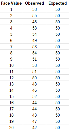
We then calculate the test statistic $\chi^2$ using the equation above, which gives us 8.56. According to statology’s chi-square score to $p$-value calculator, the $p$-value associated with $\chi^2=8.56$ and $20-1=19$ degrees of freedom is 0.980. Since 0.980 is larger than our significance level of 0.05, we fail to reject the null hypothesis that our 20-sided die follows a discrete uniform distribution.

Chi-Square Test of Independence

As mentioned, this test determines whether two variables are related to each other. A simple example can be testing for association between favorite color and favorite sport.

Again, we form our hypotheses:

• $H_0$ (null hypothesis): favorite color and sport are independent
• $H_1$ (alternative hypothesis): favorite color and sport are not independent

and define a critical value of 95% for a test of significance. Next, we interview 100 people to ask them about their favorite colors and sports. The results of the interview are provided in the tables below.

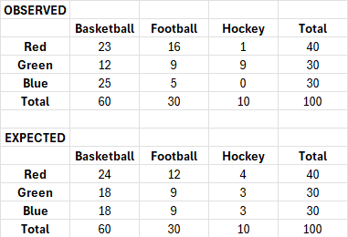
The expected count in each cell $(i,j)$ on the null hypothesis (i.e., independence holds) is

where $n=100$ is the total number of interviewees. Finally, we calculate the test statistic $\chi^2$ using the same equation used in the goodness of fit test, which gives us 25.13. The $p$-value associated with $\chi^2=25.13$ and $(3-1)\cdot(3-1)=4$ degrees of freedom is 0.000047. Since it’s much smaller than our significance level of 0.05, we reject the null hypothesis that favorite color and sport are independent.

Interpretation of $p$-values

Both chi-square tests assume a fixed but unknown true model under $H_0$ and evaluate the probability of observing data (or more extreme) given that model. In other words, the $p$-value is precisely defined as $P(\text{data or more extreme} \mid H_0 \text{ is true})$, and not $P(H_0 \text{ is true})$, which is an extremely common misconception.

I haven’t had to use any chi-square tests recently, but having lost my lecture notes (sorry, Prof), at least I’m absolutely certain I could just code the entire test from scratch if I needed to 🙂