Continuous Latent States with Kalman Filters

In the previous article, we introduced Hidden Markov Models (HMMs) as a way to capture volatility regime-switching in SPY returns. By decomposing returns into distinct states, i.e., low, medium, and high volatility, we’re able to uncover meaningful structure that a single continuous model like GARCH could not explicitly represent.

However, HMMs assume that the market operates in a finite set of discrete regimes, forcing what is inherently a continuous process into a small number of fixed states. In reality, volatility and other latent dynamics tend to evolve smoothly over time, exhibiting gradual transitions rather than abrupt switches.

To explore this idea of volatility as a continuous latent process, we turn to Kalman Filters (KFs).

***

I’ve previously detailed how KFs work to a (hopefully) comfortable degree of depth, so if you’re interested in that do check it out here. Nevertheless, some intuition, in case you’ve never seen KFs before, will be necessary.

At its core, KFs are built on a state-space model, which separates the system into two components: a hidden state and an observed measurement.

The key idea is that, like HMMs, what we observe in financial markets (i.e., prices or returns) is often a noisy manifestation of some underlying signal. While we can’t observe this state directly, we assume that it evolves continuously (whereas it would be discrete in the case of HMMs) over time according to some simple dynamics.

Formally, the model is defined by two equations. The first describes how the hidden state evolves:

where $x_t$ represents the hidden state at time $t$, and $w_t$ is random noise capturing unexpected changes in the state. This equation reduces to a random walk in the simplest case, where the state today is just yesterday’s plus some small disturbance.

The second equation links this hidden state to what we actually observe:

Here, $y_t$ is the observed data (e.g., SPY log returns) and $v_t$ represents observation noise. Basically, this reflects the idea that returns are influenced by short-term fluctuations, microstructure noise, and randomness.

Putting these together, the KF works as follows: it maintains a running estimate of the probabilistic belief about $x_t$, summarized by its mean $\hat{x}_t$ and variance $P_t$. At each time step, it:

• Predicts the next state based on past information

• Updates that estimate using the new observation

This creates a dynamic balance between trusting the model (i.e., the predicted state) and trusting the data (i.e., the observed value).

Data Preparation

Unlike GARCH and HMM, KF assumes a linear-Gaussian structure. However, squared returns violate this because they are strictly positive, skewed, and multiplicative in nature. Therefore, we instead take the log of squared returns as the volatility proxy, which makes the dynamics approximately additive and more Gaussian-like:

import numpy as np
import yfinance as yf

# Download SPY prices
spy_prices = yf.download(
    '^GSPC',
    start='2010-01-01',
    end='2025-12-31',
    auto_adjust=True,
    progress=False
)['Close'].dropna()

# Compute log returns
spy_log_rets = np.log(spy_prices / spy_prices.shift(1)).dropna()

# Transform to log-squared returns (volatility proxy)
eps = 1e-8  # small constant for numerical stability
spy_log_sq_rets = np.log(spy_log_rets**2 + eps)

# Train-test split
train = spy_log_sq_rets.loc['2010-01-01':'2019-12-31']
test  = spy_log_sq_rets.loc['2020-01-01':'2025-12-31']

Model Specification and Fitting

This time, we’ll rely on the pykalman package to fit a KF to SPY log returns. We should therefore first reshape the data to the expected input formats:

# pykalman expects shape (T, n_dim_obs)
train_obs = train.values.reshape(-1, 1)
test_obs  = test.values.reshape(-1, 1)
full_obs  = spy_log_sq_rets.values.reshape(-1, 1)

And then define the KF:

from pykalman import KalmanFilter

kf = KalmanFilter(
    transition_matrices=np.array([[1.0]]),
    observation_matrices=np.array([[1.0]])
)

By setting both the transition and observation matrices to 1.0, we’re essentially specifying a simple local-level model where the latent state follows a random walk and the observed data is a direct noisy measurement of that state.

kf = kf.em(train_obs, n_iter=100)
filtered_state_means, filtered_state_covs = kf.filter(full_obs)
smoothed_state_means, smoothed_state_covs = kf.smooth(full_obs)

kf.em() estimates the model parameters using the Expectation-Maximization (EM) algorithm on the train set, which learns the appropriate levels of state and observation noise directly from the data. With the fitted model, we run kf.filter() on the full dataset to obtain the filtered estimates, which provide causal estimates of the latent volatility using only past information.

Finally, we run kf.smooth(), which refines the filtered estimates by incorporating the entire dataset to produce a hindsight-based estimate of the underlying volatility process.

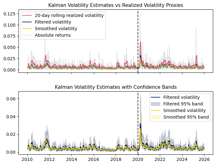
Note that the series before the dotted vertical line is the train set, while those after is the test set. Keep this in mind: the KF is trying to recover the underlying signal behind the volatility proxies, not matching their spikes.

We see that rolling realized volatility smooths the fluctuations in absolute returns but remains reactive and prone to lag. In contrast, the Kalman filtered estimate provides a more stable, model-based measure of latent volatility. The smoothed estimate further refines this by incorporating future information, yielding the most stable representation of the underlying volatility process.

Limitations

But, so what? Is the KF successful in extracting a smooth latent volatility signal?

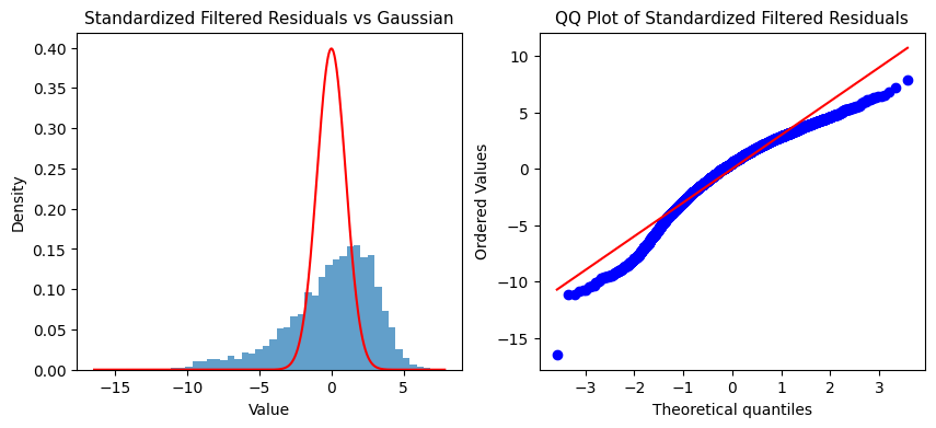
If the KF were truly successful, then the remaining signal (i.e., residuals) should be approximately Gaussian, following the idea that realized volatility equals true volatility (captured by an ideal KF) plus random noise.

However, the residuals clearly deviate from normality: the flatter peak suggests underfitting, the left skew indicates bias in volatility estimates, and fat tails reflect the model’s failure to capture extreme market moves. Overall, while the KF extracts a smooth signal, its linear-Gaussian assumptions break down in the presence of real-world asymmetry and heavy tails.

***

We’ve seen how KFs provide a powerful framework for extracting a continuous estimate of latent volatility. At the same time, our diagnostics reveal that its linear-Gaussian assumption is too restrictive for real financial data. Evidently, the model successfully captures the persistent structure of volatility, but fails to account for asymmetry, heavy tails, and extreme market movements, which are instead absorbed into its noise term.

Perhaps, then, volatility is not just a hidden state to be filtered, but a stochastic process in its own right, often exhibiting richer dynamics than a simple linear model can capture. Next time, we’ll build on this idea by introducing stochastic volatility models, where volatility evolves explicitly as a latent process, allowing us to better model the complex behavior observed in financial markets.