
Previously, we saw that modeling variance, rather than the mean, provides a much more effective way of capturing financial time series dynamics. GARCH models, in particular, are able to reproduce volatility clustering and persistence, making them a strong baseline for volatility modeling.
However, GARCH comes with an important structural assumption, which is that volatility evolves smoothly as a deterministic function of past shocks and past variance. In reality, financial markets often appear to operate in distinct regimes, with periods of sustained low volatility punctuated by sudden transitions into high-volatility environments, such as during crises.
So we simply ask: what if volatility is not just evolving continuously, but instead switching between different states? And to explore this idea, we turn to Hidden Markov Models (HMMs).
***
I’ve actually somewhat rigorously covered the theory of HMMs (check it out here), but I still want to at least cover some intuition before diving into how we use it in practice.
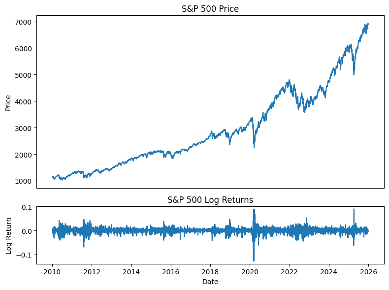
An HMM assumes that the observed data — the SPY log returns — is generated by an underlying hidden state that evolves over time. In this case, we’ll consider a 3-state HMM, meaning at each (daily) time step, we assume that the market is in one of three hidden states: low, medium, or high volatility.
The idea here is that the hidden state evolves according to a Markov process, and the probabilities of moving to some next state are captured in a transition matrix. Moreover, each state generates returns (which is what we can observe) according to a specific distribution. Altogether, at each step, the model is in some hidden state unknown to us, generates a return, then transitions to the next one, rinse and repeat until the end of the sequence.
Model Specification and Fitting
For ease of use, we’ll be referencing hmmlearn to fit an HMM to SPY log returns.
from sklearn.preprocessing import StandardScaler

X = train.values.reshape(-1, 1)
scaler = StandardScaler()
X_scaled = scaler.fit_transform(X)
We simply reshape the data to match the specific input format that hmmlearn expects. Because log returns are very tiny, we should also scale it for numerical stability during the downstream Expectation-Maximization (EM) algorithm.
from hmmlearn import hmm

model = hmm.GaussianHMM(
    n_components=3,
    covariance_type="diag",
    n_iter=1000,
    tol=1e-6,
    random_state=42,
    verbose=False
)
model.fit(X_scaled)
score = model.score(X_scaled)
Next, we define the 3-state Gaussian HMM. The model will run up to 1000 of the EM algorithm for parameter estimation, stopping early if the log-likelihood improvement falls below the tolerance of (suggesting convergence). The random state simply sets a fixed seed for reproducibility in parameter initialization.
Importantly, note that the EM step follows a Baum-Welch algorithm, which optimizes a non-convex likelihood that guarantees convergence only to a local minimum. Hence, we should aim to run the model fitting with multiple seeds (i.e., various initializations) and pick the highest scored model according to model.score(), which calculates the total log-likelihood of the observed data under the trained model.
Earlier, we assigned n_components=3 simply because it intuitively felt the most interpretable. But what if we were unsure of how many states to use? To quantify this, we could define a range of states and loop the entire fitting process across the different number of states, recording the AIC, BIC, and log-likelihood score values across the range.
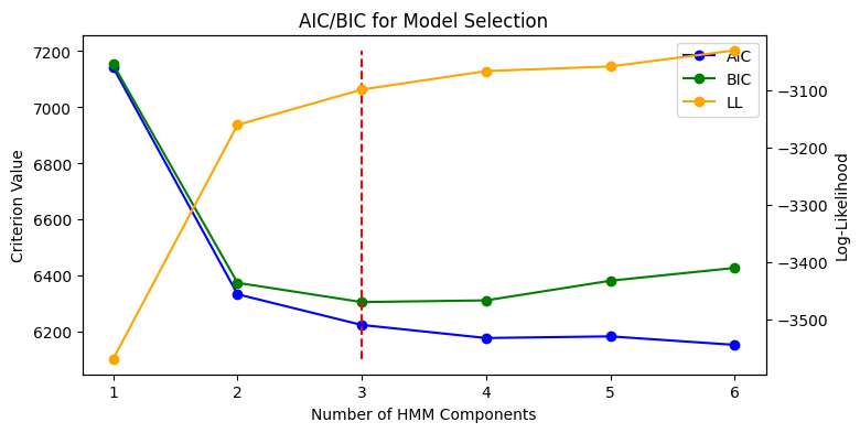
Observably, the values of the three metrics seem to point to three components being the ideal as BIC (which heavily penalized model complexity) is lowest at 3. Very nice. Once we’ve fitted the best model, we can check the model’s learned initial distribution, transition matrix, as well as the emission distribution per state.
print("Learned initial distribution:", model.startprob_)
print("Learned transition matrix:\n", model.transmat_)
print("Learned scaled means:\n", model.means_)
print("Learned scaled covariances:\n", model.covars_)
Learned start probabilities: [1. 0. 0.]
Learned transition matrix:
[[9.33465384e-01 6.47808593e-02 1.75375708e-03]
[7.00469920e-02 9.19795579e-01 1.01574294e-02]
[2.05351549e-60 3.60068055e-02 9.63993195e-01]]
Learned means:
[[ 0.0814905 ]
[-0.01128337]
[-0.22407807]]
Learned covariances:
[[[0.19751816]]
[[0.96286523]]
[[3.57978145]]]Overall, the fitted HMM reveals an interpretable volatility regime structure. The transition matrix is strongly diagonal, indicating high persistence within each state and confirming that regimes are relatively stable over time rather than rapidly switching.
Moreover, the learned means and covariances further differentiate the regimes:
- State zero exhibits small positive returns with low variance (low-volatility bullish regime),
- State one centers near zero with moderate variance (neutral or normal market conditions), and
- State two captures large negative returns with significantly higher variance (high-volatility bearish regime).
For a clear visualization of these results, we can plot the standardized distributions for each of the states as follows:
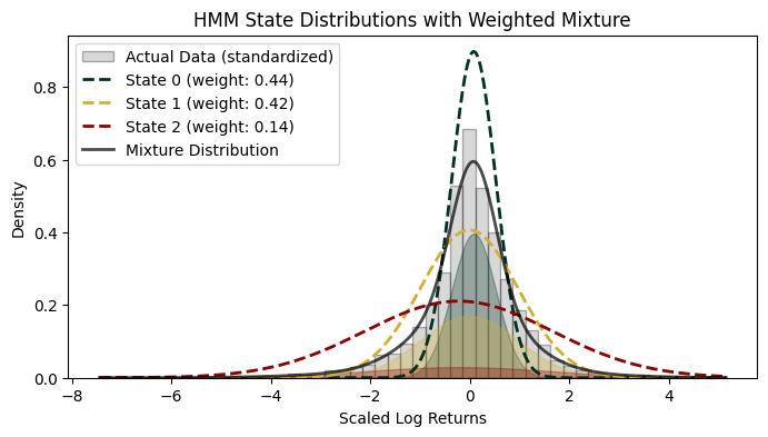
SPY log returns are well known to be non-Gaussian, exhibiting both heavy tails and negative skewness. By decomposing returns into distinct regimes, the Gaussian HMM attempts to model each regime with its own simpler, approximately Gaussian distribution that reflects the characteristics of that specific state.
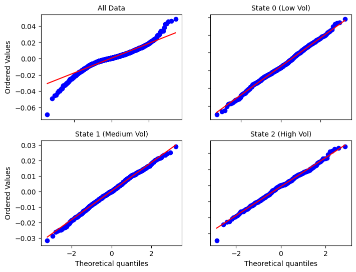
From the QQ plots, the full dataset clearly deviates from normality, particularly in the tails. However, once segmented into regimes, each subset aligns much more closely with the Gaussian reference line, indicating that the HMM has successfully decomposed a complex, non-Gaussian distribution into a mixture of simpler, near-Gaussian components.
Moving on, we can also plot what the regimes are exactly at each time point across the train period:
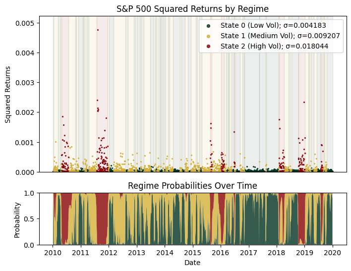
The top plot represents the Viterbi decoding (hard assignment), while the bottom shows the posterior probabilities (soft assignment) from the forward-backward algorithm in the E-step of EM. We observe that the HMM correctly identifies several economic crises as high volatility periods (e.g., the European Debt Crisis of 2011).
Out-of-Sample Inference
Now, we scale the test period using the same scaler as we have for the train set:
X_test = test.values.reshape(-1, 1)
X_test_scaled = scaler.transform(X_test)
Using the fitted model to predict the states in the test period yields the following plot:
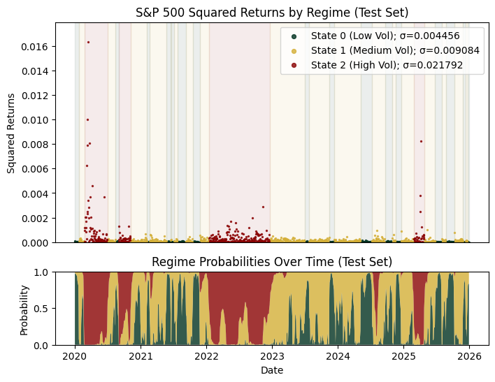
It’s very important to stress that the model.predict() function defined in the package uses Viterbi decoding and model.predict_proba() uses the forward-backward algorithm, which means that the two aren’t causal, i.e., they look at future data to predict the present state.
This implies that live state prediction is okay because the dataset we’d be using wouldn’t have future data to begin with. However, lookahead bias will be an issue for historical evaluation (i.e., during back-testing). To circumvent this, we replace the batch inference on the full test set with an expanding window approach such that at each time step , the model only sees data up to rather than the entire future path.
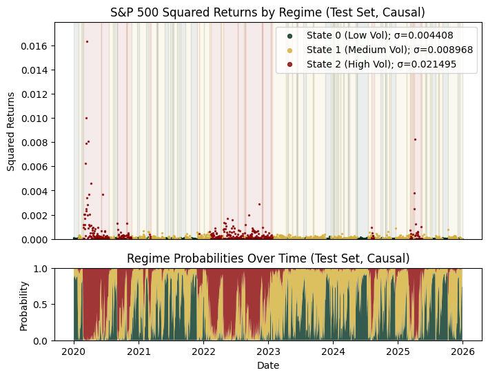
As expected, removing smoothing makes the regime probabilities appear noisier. However, the overall regime structure remains broadly consistent with the smoothed results, indicating that the model is still capturing meaningful patterns. Notably, we see that major stress periods such as the COVID-19 shock in 2020 and the overlapping macro crises in 2022 are quite clearly identified.
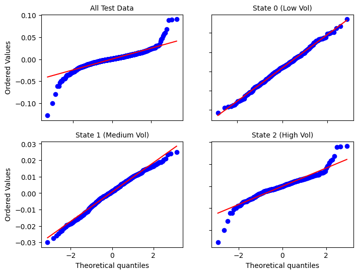
However, since the market is always changing, the dynamic of each regime in the test period may no longer look like what is expected of that regime during training. We see this discrepancy manifest very obviously in the high volatility state, where the issue of fat tails and left-skewness has reappeared. Note that the non-causal QQ plots also look similar to the above.
Limitations
Of course, HMMs aren’t perfect. In fact, the main limitations arise from its simplification (perhaps as a consequence of the bias-variance tradeoff) of temporal dependence and continuous nature of real financial dynamics.
First is the Markov assumption. It’s unrealistic for markets like SPY to have a regime transition depend only on the previous state, ignoring the duration spent in a regime. A clear manifestation of this is in the frequent regime-switching in the causal test period. While explicitly modeling duration (e.g., Hidden Semi-Markov Models (HSMMs)) is a theoretical solution, its numerical instability makes it vastly challenging to implement in practice.
An elegant fix for this is to instead apply post-processing smoothing to the inferred regimes.
st_series = pd.Series(hid_st_test, index=test.index)
hid_st_smooth = st_series.rolling(20).median()
hid_st_smooth = hid_st_smooth.fillna(method='bfill').fillna(method='ffill')
hid_st_smooth = hid_st_smooth.astype(int).values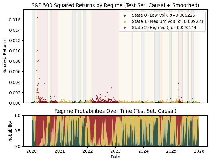
As we can see, applying a 20-period rolling median to the causal estimates produces results that closely resemble the non-causal version, while more effectively capturing regime persistence.
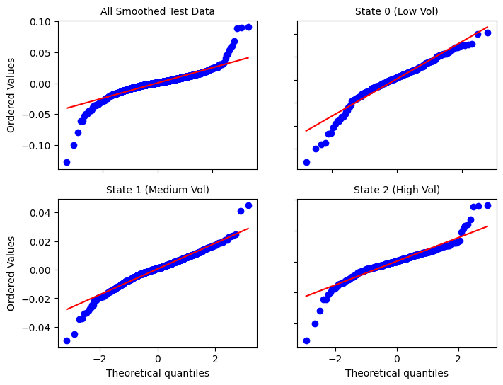
Unfortunately, this smoothing causes our approximately Gaussian-distributed regimes to deviate from normality back to the aforementioned issues of heavy-tailedness and left-skewness.
Second, HMMs assume a finite set of discrete regimes, whereas market volatility typically evolves continuously. This can force smooth changes into artificial jumps between states. Models like Kalman Filters (state-space models) address this by allowing latent variables (e.g., volatility) to evolve continuously over time rather than switching between fixed regimes.
***
While HMMs improve upon GARCH by introducing regime-switching behavior, they still treat volatility as a discrete and externally imposed structure. This naturally leads to a deeper question: what if volatility itself is a continuous, latent process that evolves independently over time? In the next articles, we’ll explore Kalman filters and stochastic volatility models, which take this idea seriously by modeling volatility as its own hidden process with richer and more realistic dynamics.
Leave a Reply