Reasoning a World We Cannot See

My fiancée has this supernatural ability she calls gut feeling where she’s able to somewhat accurately able to sense a hidden truth. The other day, she told me out of the blue that she felt a little nauseous, and then out of the blue, that perhaps so-and-so we’re broken up. Then we’d stalk their socials and find her words true.

Okay, now I’m not so insane that every single life experience becomes a lesson on statistics, but I thought this would make a smooth segue (fun fact: you probably thought this was spelled segway) into Hidden Markov Models (HMMs), one of the coolest topics I’ve ever encountered.

If we had to quantify “woman’s intuition,” doesn’t it look a lot like gut feeling becomes some observable state which predicts some hidden state, say whether so-and-so and his girlfriend were still together? Anyway, this unserious introduction isn’t a reflection of the quality of the content we’re about to go through.

***

Hopefully, you’ve at least heard about the Markov property, which at its core is a statement about conditional independence: the future is independent of the past, given the present. Formally, for a sequence of random variables $X_1, X_2, …, X_T$, the Markov property states that

In other words, the present already encodes everything the future cares about.

This property gives birth to a Markov chain, which is a sequence of states where each state is connected to the next by a probabilistic dependency. We can think of it as a directed graph whose edges carry probabilities, and where the process “hops” from node to node over time.

Now that we’ve accepted the Markov property, we need a concrete way to describe how the process moves between states. Suppose the system can occupy one of $N$ states $\mathcal{S}=\{s_1,s_2,…,s_N\}$. Then, the transition dynamics are fully captured by the transition probability matrix $A$, where each entry is defined as

$A$ is an $(N \times N)$ matrix with each row summing to one, since the system must go somewhere:

This matrix is basically the complete specification of how the hidden world evolves over time. If we know the current state and we know $A$, then we know everything there’s to know about the future distribution of the chain. To connect to the idea of the Markov property: there’s no need to look back.

Now, let’s consider an interesting example where we’ll see that the plain Markov chain becomes insufficient for many real-world problems.

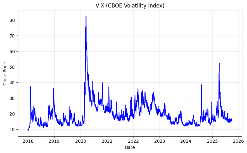
Consider the CBOE Volatility Index (VIX), a time series of market volatility readings. Economists often speak of the market being in a low volatility regime or a high volatility regime, with occasional transitions between them. These regimes are economically meaningful given they reflect the collective uncertainty of market participants. But crucially, we never directly observe which regime the market is in. Instead, we only see the VIX values themselves (see the above plot)—noisy and continuous numbers.

The fundamental problem is that the states that govern the dynamics are hidden. What we observe are not the states themselves, but signals called emissions produced by those states.

Given the states themselves are unknown, the standard Markov chain is not equipped for this setting because it assumes states are directly observed. It’s clear that we need a richer model: one with two distinct layers of randomness.

An HMM is defined exactly by this two-layer structure:

• The Hidden layer is an unobserved Markov chain over states $\mathcal{S}=\{s_1,…,s_N\}$, governed by the transition matrix $A$ and an initial state distribution $\pi$, where $\pi_i = P(X_1 = s_i)$. This layer evolves according to the Markov property but we simply can’t see it.
• The Observable layer is such that at each time step $t$, the hidden state $X_t$ produces an observable $Y_t$ according to an emission distribution $B$, defined as

The emission distribution can be discrete (e.g., a categorical distribution) or continuous (e.g., Gaussian), depending on the application. Gaussian emissions are natural for the VIX example (because of geometric Brownian motion—a topic for another day!) where each volatility regime has its own mean and variance: a calm regime samples from $\mathcal{N}(\mu_{\text{low}}, \sigma_{\text{low}}^2)$ while a turbulent one samples from $\mathcal{N}(\mu_{\text{high}}, \sigma_{\text{high}}^2)$.

This way, we acknowledge that the complete HMM is specified by three objects:

This triplet fully defines the joint distribution over both the hidden state sequence $\mathbf{X} = (X_1, …, X_T)$ and the observation sequence $\mathbf{Y} = (Y_1, …, Y_T)$:

This factorization is easier than it looks. The first term basically places us in an initial state. The product over $b_{x_t}(y_t)$ says that each state independently generates its observation. Simultaneously, the product over $a_{x_{t-1}, x_t}$ chains the states together via the Markov property.

Now that we have a model, we can begin to ask the central inferential question: given the observations $\mathbf{Y}$, what can we say about the hidden states $\mathbf{X}$? This is precisely a posterior inference problem, and therefore Bayes’ theorem is the natural lens for us to view this:

where each term conveniently has a direct interpretation in the HMM framework:

• $P(\mathbf{X} \mid \lambda)$ is the prior over state paths, encoded by the transition probabilities $A$ and the initial distribution $\pi$. It says how likely a given sequence of hidden states is before we see any data.
• $P(\mathbf{Y} \mid \mathbf{X}, \lambda)$ is the likelihood, encoded by the emission probabilities $B$. It says how well the observations are explained by a particular hidden path.
• $P(\mathbf{Y} \mid \lambda)$ is the marginal likelihood, which is the probability of the observed data under the model, integrated over all possible hidden paths.

Therefore, an HMM is not just a probabilistic graphical model, but also a Bayesian inference problem over sequences. The transition matrix is the prior, the emission model is the likelihood, and our goal is the posterior. The challenge, as we’ll see, is computational.

Suppose we have a sequence of length $T$ over $N$ states. Then, the number of possible hidden state sequences is exactly $N^T$. A naive approach to computing $P(\mathbf{Y} \mid \lambda)$ would be to enumerate all state sequences, compute each joint probability $P(\mathbf{X}, \mathbf{Y} \mid \lambda)$, and sum them up:

This is the right formula, but it’s computationally catastrophic! A different approach is therefore needed.

The key insight is in realizing that the Markov property enables dynamic programming: instead of computing the probability of each full path from scratch, we can build up probabilities incrementally, reusing partial computations.

First, we define the forward variable as

This represents the probability of having observed the first $t$ observations and being in state $s_i$ at time $t$. It can be computed recursively:

• Initialization: $\quad \alpha_1(i) = \pi_i \cdot b_i(y_1)$
• Recursion: $\quad \alpha_{t+1}(j) = b_j(y_{t+1}) \sum_{i=1}^{N} \alpha_t(i)\, a_{ij}$

Here, at each step, we extend forward from all states at time $t$ to state $j$ at time $t+1$. Because of the Markov property, the recursion is exact, meaning no information is lost by discarding the full history. Using this approach drops the total complexity from $\mathcal{O}(N^T)$ to $\mathcal{O}(N^2 T)$: polynomial, not exponential.

Now that we know about dynamic programming, let’s address three canonical problems that the HMM framework addresses.

The first is the problem of evaluation: what’s the probability of the observations? Tackling this question is done using the Forward algorithm, where given a model $\lambda$ and an observation sequence $\mathbf{Y}$, we compute $P(\mathbf{Y} \mid \lambda)$. Using the forward variable $\alpha_t(i)$, the answer is simply

This is useful for model comparison and anomaly detection.

The second is the problem of decoding: what’s the most probable hidden path? To do this, we use the Viterbi algorithm: compare the joint probabilities of the entire path sequence and observation sequence. The path sequence that yields the highest probability is the likeliest sequence. In math-speak, calculate

Using recursion,

By backtracking through the maximizing arguments, we recover the optimal state sequence. This gives us regime labels. For the VIX example, the label for each day is the volatility regime (i.e., one of low, medium, or high volatility).

Decoding also comes in softer variants:

• Filtering: estimating the current state $P(X_t \mid Y_{1:t})$, which is useful for real-time inference.
• Smoothing: estimating a past state $P(X_t \mid Y_{1:T})$ using the full sequence, which is more accurate but also requires all data.

The third is a problem of learning: how do we estimate the model parameters? In practice, the model parameters $\lambda = (A, B, \pi)$ are unknown and must be estimated from data. A popular method for this is the Baum-Welch algorithm, which is an Expectation-Maximization (EM) algorithm. Essentially, in the E-step, it uses the forward-backward algorithm to compute the expected number of transitions and emissions under the current parameters. Then, in the M-step, it re-estimates $A$, $B$, and $\pi$ to maximize the expected log-likelihood. The procedure iterates until convergence, climbing the likelihood surface without ever explicitly enumerating hidden paths.

Now I know we didn’t delve too deep into how HMM solves the problems of evaluation, decoding, and learning. Putting too much of their explanation here might shift the topic toward algorithm derivation rather than conceptual understanding. If this is something you’d love for me to get into more, do let me know! Otherwise, may you leave this article with a newfound understanding of this wonderful framework anyway.