GARCH Sees What ARIMA Cannot

In the previous article, we fit AR, MA, ARMA, and ARIMA models to SPY log returns and watched them systematically fail in a very specific way. The residuals showed volatility clustering, the QQ plots showed fat tails, and ACF plot on squared residuals confirmed that the variance itself was autocorrelated. ARIMA models the conditional mean. The problem is in the conditional variance. That’s what ARCH and GARCH are built for, and that’s we’ll explore today.

***

The data we’ll be using here is exactly the same as what we’ve used in the previous article — SPY log returns from the start of 2010 all the way to the end of 2025, with an elusive nuance: we’ll demean the log returns. We can handle this manually by running

train_demeaned = train - train.mean()

or have it handled when initializing the ARCH and GARCH models using the arch package.

Why? ARCH and GARCH models the conditional variance of the error term, i.e., the unexplained residual after accounting for the mean. If we don’t demean, we’re technically modeling the variance of returns around zero rather than around their true mean, which is a mild misspecification.

ARCH Order Selection

Before fitting, we need to determine the lag order $q$ for the ARCH($q$) model. Just as ACF/PACF of raw log returns informed mean model selection in the previous article, here we apply them to squared returns, which is our proxy for variance.

from statsmodels.graphics.tsaplots import plot_acf, plot_pacf

plot_acf(train ** 2, lags=60, ax=axes[0], color='steelblue', zero=False)
plot_pacf(train ** 2, lags=60, ax=axes[1], color='steelblue', zero=False, method='ywm')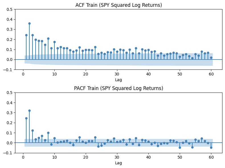

Notice that the ACF plot shows many significant spikes decaying over higher lags, indicating that today’s covariance is correlated with variance many lags into the past, and that correlation decays slowly. This is actually the key practical weakness of pure ARCH models: they require a large number of parameters to capture what is essentially long memory in variance. The ACF is telling us the model will be over-parameterized before it’s fully specified.

On the other hand, the PACF lag cutoff suggests the direct effect of past squared returns on current variance becomes negligible after lag 3, i.e., the higher-lag ACF correlations are largely mediated through intermediate lags.

from arch import arch_model

# use mean='Zero' if train is already demeaned
arch_model = arch_model(train * 100, mean='Constant', vol='ARCH', p=3)
arch_fit = arch_model.fit(disp='off')
print(arch_fit.summary())

Note that we use train * 100 instead of just train because the arch library is sensitive to the scale of the input. This way, the coefficients will need to be divided by 100 for proper interpretation. Now, let’s pay particular attention at this section of the report:

                                Mean Model                                
==========================================================================
                 coef    std err          t      P>|t|    95.0% Conf. Int.
--------------------------------------------------------------------------
mu             0.0807  1.509e-02      5.348  8.879e-08 [5.112e-02,  0.110]

                            Volatility Model                            
========================================================================
                 coef    std err          t      P>|t|  95.0% Conf. Int.
------------------------------------------------------------------------
omega          0.3057  3.102e-02      9.856  6.462e-23 [  0.245,  0.366]
alpha[1]       0.1965  4.462e-02      4.404  1.063e-05 [  0.109,  0.284]
alpha[2]       0.2958  4.565e-02      6.480  9.158e-11 [  0.206,  0.385]
alpha[3]       0.2313  4.574e-02      5.055  4.293e-07 [  0.142,  0.321]
========================================================================

First, we see a statistically significant small mu under the mean model, which suggests that SPY has a small but real positive daily drift. This is consistent with what we saw in the ARIMA article.

In the variance equation, the three alpha coefficients sum up to a high 0.724, meaning a large fraction of today’s variance is explained by just the last three shocks, with no decay mechanism. The model has no way to capture the slow, persistent variance memory the ACF showed — it can only look back three steps. Moreover, the previous ACF plot points to a long-memory process in the variance, indicating that a model capable of capturing such persistence may be more appropriate.

GARCH(1,1)

Empirically, GARCH(1,1) is hard to beat — higher-order models rarely improve fit, often introduce insignificant parameters, and add unnecessary complexity, since one shock term and one persistence term already capture the volatility dynamics.

While comparing the AIC and BIC values for several combinations of $p$ and $q$, I actually found that the AIC for GARCH(2,1) is higher than GARCH(1,1). However, the summary statistics showed that the second alpha term isn’t statistically significant. In other words, we’ll still be sticking to the historically superior GARCH(1,1) model. Below, we fit the GARCH(1,1) model the train data:

garch11 = arch_model(
    train * 100, mean='Constant', vol='GARCH',
    p=1, q=1, dist='normal'
)
garch11_fit = garch11.fit(disp='off')
print(garch11_fit.summary())

And we present its summary:

                                Mean Model                                
==========================================================================
                 coef    std err          t      P>|t|    95.0% Conf. Int.
--------------------------------------------------------------------------
mu             0.0789  1.399e-02      5.644  1.665e-08 [5.152e-02,  0.106]

                              Volatility Model                              
============================================================================
                 coef    std err          t      P>|t|      95.0% Conf. Int.
----------------------------------------------------------------------------
omega          0.0368  8.293e-03      4.443  8.879e-06 [2.059e-02,5.310e-02]
alpha[1]       0.1712  2.503e-02      6.837  8.071e-12     [  0.122,  0.220]
beta[1]        0.7898  2.429e-02     32.516 6.409e-232     [  0.742,  0.837]
============================================================================

$\alpha$ represents the shock impact (how much yesterday’s surprise moves today’s variance) and $\beta$ the variance persistence (how much yesterday’s variance carries into today). Importantly, $\alpha+\beta=0.961$ indicates highly persistent volatility, meaning shocks decay slowly (if $\alpha+\beta=1$, the process becomes IGARCH). Since $\beta\gg\alpha$, we conclude that volatility is driven more by past variance than new shocks, reflecting persistent market regimes rather than isolated spikes.

Let’s look at the diagnostic plots after fitting GARCH(1,1) on the train set:

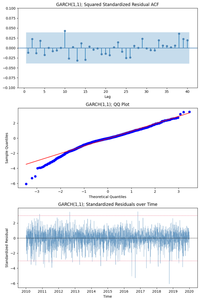
We can see that GARCH(1,1) is a much better fit from a simple AR(5) model from the previous article. First, it successfully captures the main conditional heteroskedastic structure (and therefore also the volatility clustering phenomenon), as evidenced by the lack of significant autocorrelation in the ACF plot. Moreover, the standardized residuals are centered around zero and appear largely patternless over time, indicating an adequate fit.

However, the model still isn’t perfect. The QQ plot shows a downward deviation in the lower tail, and the residual series exhibits more pronounced negative spikes, suggesting heavier left-tail behavior and possible asymmetry not fully captured under the normal error assumption.

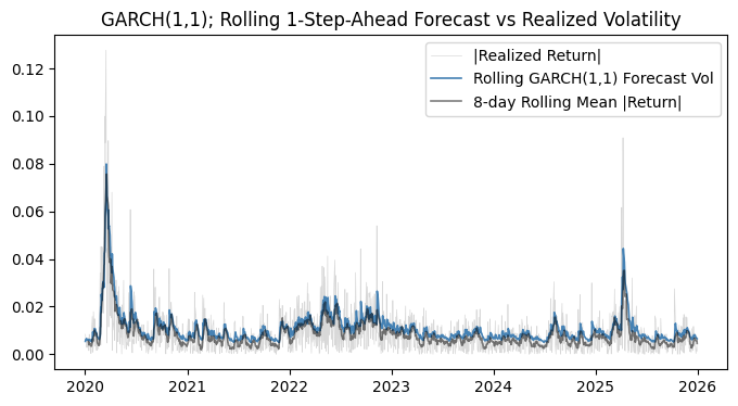
This prediction result is likely the most telling evidence that GARCH(1,1) captures the overall volatility dynamics in SPY reasonably well. It models the volatility clustering behavior nicely, although it also systematically underestimates returns. Granted, its forecasts tend to appear lower than realized absolute returns because it estimates conditional volatility, not individual shocks. This underestimation is amplified by heavy downside tails in the data, which violate the Gaussian error assumption and lead to missed extreme negative moves.

GARCH Variants

The limitations of GARCH point to the probable need to apply more sophisticated methods to model SPY log returns. We consider several direct extensions of the GARCH model to tackle these issues:

• GJR-GARCH adds an asymmetry term to capture the leverage effect: bad news hits volatility harder than good news.
• EGARCH also captures asymmetry but models the log of conditional variance instead of the variance directly.
• Student-t errors change the error distribution. Instead of assuming shocks are Gaussian, we allow for fat tails via the degrees-of-freedom parameter $\nu$, where lower $\nu$ means fatter tails.

The code below fits several combinations of GARCH models to the train set:

garch_fit = arch_model(
    train * 100, mean='Constant', vol='GARCH', p=1, q=1, dist='normal'
).fit(disp='off')
gjr_fit = arch_model(
    train * 100, mean='Constant', vol='GARCH', p=1, q=1, o=1, dist='normal'
).fit(disp='off')
egarch_fit = arch_model(
    train * 100, mean='Constant', vol='EGARCH', p=1, q=1, dist='normal'
).fit(disp='off')
garch_t_fit = arch_model(
    train * 100, mean='Constant', vol='GARCH', p=1, q=1, dist='t'
).fit(disp='off')
gjr_t_fit = arch_model(
    train * 100, mean='Constant', vol='GARCH', p=1, q=1, o=1, dist='t'
).fit(disp='off')
egarch_t_fit = arch_model(
    train * 100, mean='Constant', vol='EGARCH', p=1, q=1, dist='t'
).fit(disp='off')

We then compute the AIC/BIC values, the Ljung-Box test $p$-values, and the forecast RMSE to compare the fitness and performance of the models. The results are provided in the table below:

           Model       AIC     BIC  LB p-val     RMSE
-----------------------------------------------------
GJR-GARCH(1,1,1)-t 5738.27 5773.25    0.8644 0.003595
      GARCH(1,1)-t 5848.88 5878.03    0.8687 0.003595
     EGARCH(1,1)-t 5857.28 5886.43    0.8120 0.003421
  GJR-GARCH(1,1,1) 5889.14 5918.29    0.8711 0.003386
        GARCH(1,1) 6018.16 6041.48    0.8876 0.003169
       EGARCH(1,1) 6036.56 6059.88    0.8120 0.003245

Observably, allowing for asymmetry and heavy-tailed innovations materially improves the statistical fit, with the GJR-GARCH(1,1)-t specification emerging as the clear in-sample winner based on AIC and BIC. This confirms that both the leverage effect and fat tails are important features of SPY log return dynamics that a symmetric, Gaussian GARCH model fails to capture.

However, we note that these improvements don’t actually meaningfully translate into better out-of-sample forecasts. Across all specifications, forecast RMSE remains remarkably similar, with even the simple GARCH(1,1) performing competitively. We highlight a key empirical insight: while richer GARCH variants better describe the distribution of returns, short-term volatility forecasts are largely driven by persistence, meaning additional complexity often yields diminishing returns in predictive performance.

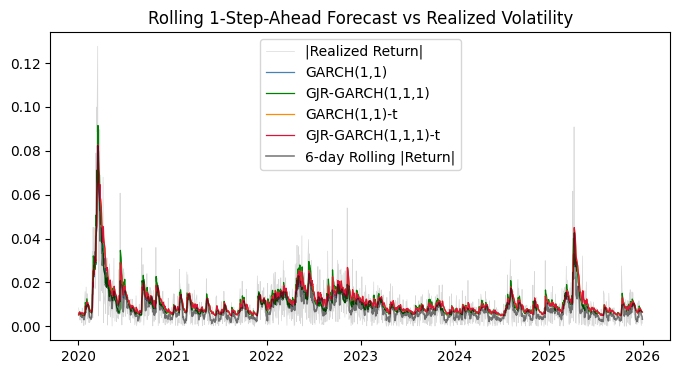
Visualizing the 1-step-ahead forecasts yields a similar story: there isn’t much difference between the various models and model extensions, which suggests that the simplest GARCH(1,1) may be sufficient for a prediction task given our data.

***

As we’ve seen, modeling variance is far more effective than modeling the mean in capturing financial time series dynamics. However, GARCH(1,1) remains limited because it assumes a symmetric response to shocks despite well-known leverage effects, and its default Gaussian assumption fails to account for fat tails. As a solution to this, we adopted several extensions of GARCH and observed a considerable improvement in statistical fit, although the GARCH remained competitive in predictive scenarios.

In the next article, we move beyond the GARCH framework altogether. Rather than treating volatility as a deterministic function of past shocks, we’ll explore models where volatility evolves more dynamically either through discrete regime changes using Hidden Markov Models, or as a latent stochastic process in stochastic volatility models.