Penalized Regression for Stock Returns

Predicting asset returns is a difficult game where the usual rules of regression are stress-tested by noisy signals, correlated features, and the ever-present risk of overfitting to market microstructure. While ordinary least squares (OLS) gives us a clean starting point, penalized regression methods like Ridge, LASSO, and Elastic Net offer a principled way to impose structure on that noise.

Note that due to the violation of assumptions, the performances of the models will suck a lot. The goal is therefore to understand how regularization changes what a model learns, what it discards, and how we should think about bias-variance tradeoff in a low-signal financial setting (i.e., not to build a trading strategy).

***

Throughout this blog, we’ll be walking through a progression of regression models applied to daily AAPL returns using five technical indicators as features:

Feature	Description
momentum_rsi	Strength of recent gains vs losses
trend_macd_diff	Difference between MACD and signal line
volatility_atr	Average daily price range (incl. gaps)
volume_mfi	RSI weighted by volume (money flow)
trend_adx	Strength of a trend (no direction)
trend_sma_fast	Short-term simple moving average
trend_sma_slow	Long-term simple moving average
trend_ema_fast	Short-term exponential moving average
trend_ema_slow	Long-term exponential moving average
target	Daily Return (Prediction Target)

For now, we’ll split our data to train and test sets:

from sklearn.model_selection import train_test_split

X = aapl_.drop(columns="target")
y = aapl_["target"]
X_train, X_test, y_train, y_test = train_test_split(
    X, y, test_size=0.2, shuffle=False
)

Linear Regression (OLS Baseline)

OLS is a supervised, parametric linear regression method belonging to the family of generalized linear models (GLMs) that assumes the data generating process to follow

Our objective here is to estimate the coefficient vector $\boldsymbol{\beta}$, $\hat{\boldsymbol{\beta}}$, that minimizes the discrepancy between observed and predicted values, otherwise known as the sum of squared residuals:

which has the closed form solution:

Having a closed form solution means that no iterative optimization is needed (because the answer is directly computed), making the calculation fast and deterministic. Moreover, OLS coefficients have an intuitive interpretation: a one unit increase in $x_i$ produces a $\hat{\beta}_i$ change in $\hat{y}$.

We can fit a simple linear regression by calling the LinearRegression class from the scikit-learn package.

from sklearn.linear_model import LinearRegression

ols = LinearRegression()
ols.fit(X_train, y_train)
y_train_pred = ols.predict(X_train)
y_pred = ols.predict(X_test)

Evaluating the metrics, we obtain an $R^2$ and MSE value of 0.0027 and 0.000320, as well as -0.0192 and 0.000289 for the train and test sets, respectively. The most glaring red flag here is how low the $R^2$ values are, but these are not unexpected.

The main culprit is model misspecification, which occurs because several assumptions of the model input are violated by our data. This is where we move on to penalized regression models, in hopes that we can salvage the results by fitting a model that better reflects the assumptions of the data.

Ridge Regression

Like OLS, Ridge regression is a continuous, non-sparse estimator. Unlike OLS, it adds an $\ell_2$ penalty to shrink coefficients toward zero without eliminating them:

which also has the closed-form solution:

In eigenvalue terms, by adding $\lambda \mathbf{I}$ to $\mathbf{X}^\top \mathbf{X}$, we’re preventing two highly correlated predictors from having an eigenvalue that’s very close to zero because it’s now bounded below by $\lambda$. This is clearly explained from the Singular value decomposition (SVD) perspective (letting $\mathbf{X}=\mathbf{UDV}^\top$):

where $d_j$ are singular values. We see that Ridge shrinks each component by the factor $\frac{d_j^2}{d_j^2 + \lambda}$, meaning directions with small singular values (often variables exhibiting multicollinearity) are shrunk most aggressively.

So when do we want to consider Ridge? Among other reasons, it’s typically appropriate on a dense signal assumption (i.e., many predictors are expected to carry some signal), when predictors are correlated and we want to retain all of them, and when the interpretability of individual coefficients matters less than predictive stability for the task.

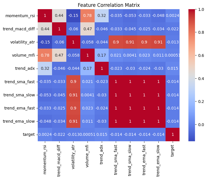
This should be beneficial for our dataset, given how the SMA and EMA features are very highly correlated with one another and the average true range, and we don’t want to remove all these predictors.

from sklearn.preprocessing import StandardScaler
from sklearn.linear_model import Ridge

# Standardize data
scaler = StandardScaler()
X_train_sc = scaler.fit_transform(X_train)
X_test_sc  = scaler.transform(X_test)

# Fit Ridge
ridge = Ridge(alpha=2.0)
ridge.fit(X_train_sc, y_train)
y_train_pred_ridge = ridge.predict(X_train_sc)
y_pred_ridge = ridge.predict(X_test_sc)

Note that for now, I’ve decided to heuristically assign alpha=2.0. In reality, this term is basically $\lambda$, which is a hyperparameter that needs to be tuned according to the data. Here, we obtain an $R^2$ and MSE value of 0.0013 and 0.000320, as well as -0.0078 and 0.000286 for the train and test sets, respectively. We’ll compare the metrics and coefficients from all the models in a later section.

LASSO Regression

The Least Absolute Shrinkage and Selection Operator (LASSO) regression replaces the $\ell_2$ penalty with an $\ell_1$ penalty:

The $\ell_1$ norm induces sparsity, meaning unlike Ridge, it drives particular coefficients to exactly zero, thereby performing automatic feature selection. Also, unlike OLS and Ridge, LASSO has no analytical solution because $|\beta_j|$ at zero is non-differentiable (i.e., requires iterative optimization).

Interestingly, multicollinearity becomes a problem here once again. When predictors are correlated (e.g., the four SMA/EMA features), LASSO arbitrarily selects one and zeros out the reset. The issue is that the choice of which to keep is sensitive to small data perturbations. In the context of financial returns, which is notoriously noisy, this sensitivity becomes somewhat worrisome.

Almost quite the “opposite” of the Ridge counterpart, we usually consider fitting LASSO when only a subset of predictors carry signal (i.e., sparsity is expected), feature selection and estimation are to be done simultaneously, and when an interpretable model is preferred over retaining all features.

from sklearn.linear_model import Lasso

lasso = Lasso(alpha=0.0001, max_iter=10000)
lasso.fit(X_train_sc, y_train)
y_train_pred_lasso = lasso.predict(X_train_sc)
y_pred_lasso = lasso.predict(X_test_sc)

Because LASSO essentially zeros out features it considers “not worth keeping,” running this unsurprisingly drops most of the predictors, leaving behind only volatility_atr, volume_mfi, trend_adx. With this, we obtain an $R^2$ and MSE value of 0.0007 and 0.000321, as well as -0.0018 and 0.000285 for the train and test sets, respectively.

Elastic Net

The Elastic Net merges the best of both worlds, Ridge and LASSO, by combining both $\ell_1$ and $\ell_2$ penalties, thereby inheriting Ridge’s grouping stability and LASSO’s sparsity:

This is actually typically reparameterized using a mixing parameter $\rho \in [0, 1]$:

where $\rho = 1$ indicates pure LASSO, $\rho = 0$ indicates pure Ridge, and anything in between the Elastic Net.

It’s appropriate when predictors are moderately to highly correlated, when the true signal is expected to be sparse but not extremely so, and when LASSO’s instability under correlation is a practical concern (which, as we’ve seen, is the case with financial technical indicators).

from sklearn.linear_model import ElasticNet

en = ElasticNet(alpha=0.0001, l1_ratio=0.5, max_iter=10000)
en.fit(X_train_sc, y_train)
y_train_pred_en = en.predict(X_train_sc)
y_pred_en = en.predict(X_test_sc)

Like all the previous parameterized models, we’ve also used heuristically determined values for the parameters alpha and l1_ratio. The results of the fitting will therefore, like the rest, be unoptimal, which is why we’ll skip the metrics and move on to the next very important step: hyperparameter tuning.

Hyperparameter Tuning

By now, we understand that all three penalized models — Ridge, LASSO, and Elastic Net — introduce at least one regularization hyperparameter that isn’t learned from the data during fitting. By poorly choosing a set of such values, the models very commonly underfit or overfit. Therefore, the goal of hyperparameter tuning is to find the values that generalize best to unseen data using cross-validation.

from sklearn.model_selection import GridSearchCV, TimeSeriesSplit

tscv = TimeSeriesSplit(n_splits=5)

param_grid = {
    "alpha"   : [0.0001, 0.001, 0.01, 0.1],
    "l1_ratio": [0.1, 0.3, 0.5, 0.7, 0.9, 0.95, 1.0]
}

gs = GridSearchCV(
    ElasticNet(max_iter=10000),
    param_grid,
    cv=tscv,
    scoring="neg_mean_squared_error",
    n_jobs=-1,
    verbose=1
)
gs.fit(X_train_sc, y_train)

First, we use TimeSeriesSplit() to split the train data while preserving temporal temporal order. By setting n_splits=5, we’re essentially doing a 5-fold cross validation. We then run a grid search which exhaustively evaluates every combination in the predefined hyperparameter grid. It’s the right starting point because it gives a structured, interpretable map of the loss surface across a wide range.

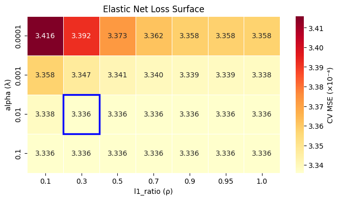
Because the MSE of the combinations when alpha=0.01 or alpha=0.1 is identical and lowest for most l1_ratio, it arbitrarily picked one combination, which, in this case, happens to be alpha=0.01 and l1_ratio=0.3, as annotated by the blue box.

Let’s plug these values back into the Elastic Nets model and rerun the fit:

en_tuned = ElasticNet(alpha=0.01, l1_ratio=0.3, max_iter=10000)
en_tuned.fit(X_train_sc, y_train)
y_train_pred_en_tuned = en_tuned.predict(X_train_sc)
y_pred_en_tuned = en_tuned.predict(X_test_sc)

Performance Comparison Analysis

Finally, we compare the performance metrics of all the previous models, including the tuned Elastic Net:

   Model    Tr R²     Te R²   Tr MSE   Te MSE  Tr/Te MSE  Non-zero Coefs
------------------------------------------------------------------------
OLS      0.002693 -0.019178 0.000320 0.000289     1.1057               9
Ridge    0.001253 -0.007802 0.000320 0.000286     1.1198               9
LASSO    0.000661 -0.001808 0.000321 0.000285     1.1272               3
EN       0.000888 -0.003284 0.000321 0.000285     1.1253               4
EN_tuned 0.000000 -0.000148 0.000321 0.000284     1.1298               0

Notice how every model produces a near-zero train $R^2$ and a negative test $R^2$, meaning each performs worse out-of-sample than simply predicting the mean return for every observation, i.e., using the null model. This isn’t surprising (and isn’t a failure of methodology), given it reflects the well-documented near-unpredictability of short-horizon equity returns from technical indicators alone.

Interestingly, we also observe the bias-variance tradeoff theory play out here: as we constrain the model further with additional penalties (i.e., OLS → Ridge → LASSO → tuned Elastic Net), train $R^2$ falls monotonically while test $R^2$ improves towards zero.

The train-to-test MSE ratios sitting just above 1.1 across all models tell us that underfitting persists, meaning they’re failing to find signal that generalizes the structure of returns. This is further confirmed by the tuned Elastic Net, which zeros out all coefficients entirely and produces the best test MSE of all five models.

Lastly, the sparsity progression (i.e., OLS retaining all 9 parameters, LASSO retaining 3, Elastic Net 4, and the tuned model retaining none) suggests that if any signal exists at all, it’s concentrated in a small subset of indicators. However, given the $R^2$ values, even those retained coefficients are more likely capturing noise than genuine predictive structure.

***

At the end of the day, no amount of regularization can conjure signal that isn’t there. We’ve just seen OLS, Ridge, LASSO, and Elastic Net all explain that daily AAPL returns aren’t linearly predictable from these technical indicators, and the most honest model turned out to be the one that predicted the mean and called it a day.

That said, the progression from OLS to penalized regression is worth understanding deeply simply because it gives us a principled, transparent framework for handling noise, multicollinearity, and overfitting that’ll matter enormously when better features or richer data are on the table.

Basically, think of this as the foundation, not the ceiling.