When Variance Has a Memory

Every ARIMA model that we write carries an assumption we might not have explicitly stated. When we consider the error term $\varepsilon_t$, we assume that

where $\sigma^2$ is a constant. We call this homoskedasticity, and for many applications, it’s honestly reasonable enough. However, some data (e.g., financial time series) have a well-documented habit of violating it.

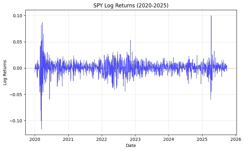
Take a look at the plot for the S&P 500’s log returns above. It’s clear that the magnitude of daily swings isn’t constant across time. We observe that markets go through stretches of relative calm (e.g., mid-2023 to mid-2024) and then abruptly enter periods where large moves happen day after day (e.g., early 2020). This phenomenon is called volatility clustering: large changes tend to be followed by large changes, and small changes tend to be followed by small changes.

If we fit ARIMA to this data and square the estimated residuals (a rough proxy for realized variance) and plot their autocorrelation function, we’ll find significant positive autocorrelation at multiple lags. In other words, the squared errors are not serially independent and so there must be some structure in the variance that ARIMA completely ignored.

Basically, the noise itself has memory. And we need a model that respects that.

***

We call the ARIMA model a mean equation, meaning it models the expected value of $r_t$ conditional on the past. What we’re going to do is recognize that the residuals from that mean equation have their own dynamics, and build a variance equation to describe them.

Concretely, if the mean equation gives us

where $\mu_t$ is the ARIMA-fitted conditional mean, then instead of treating $\varepsilon_t$ as simple white noise, we’ll write

As we can see, the innovation $\varepsilon_t$ is decomposed into a time-varying scale $\sigma_t$ (the conditional standard deviation) and a standardized i.i.d. shock $z_t$. Hereon, our job is to model how $\sigma_t^2$, the conditional variance, evolves over time.

Unconditional vs. Conditional Variance

Before introducing the models, let’s be precise about what “conditional” means here, because the terminology can be confusing. The unconditional variance of $\varepsilon_t$ is just the long-run, time-averaged variance. It’s essentially the single number $\sigma^2$ that classical models assume is constant throughout which aims to answer the question: on average, across all of time, how variable is this series?

On the other hand, conditional variance, written $\sigma_t^2 = \text{Var}(\varepsilon_t \mid \mathcal{F}_{t-1})$, is a forecast of tomorrow’s variance given everything we know up to and including today (i.e., the information set $\mathcal{F}_{t-1}$). It answers the question: given what just happened in the market, how volatile should I expect tomorrow to be?

I want to stress that although this sounds a lot like Bayesian reasoning, it actually isn’t because there’s no prior distribution being updated here. This is the frequentist conditional expectation where we’re simply allowing the variance to be a function of the observable past, in the same way that an AR model allows the mean to be a function of the observable past.

Basically, the conditional variance moves around, and that movement is exactly what we want to capture.

Autoregressive Conditional Heteroskedasticity (ARCH)

The Autoregressive Conditional Heteroskedasticity (ARCH) model is the natural starting point. The ARCH($q$) model specifies the conditional variance as a linear function of the $q$ most recent squared residuals:

with the constraints $\omega > 0$ and $\alpha_i \geq 0$ for all $i$, which ensure the variance stays positive. The analogy to an AR($q$) model is precise: just as an AR model says that today’s level depends on $q$ past levels, ARCH says that today’s variance depends on $q$ past squared shocks.

If there was a large shock yesterday (i.e., a big market move), then $\varepsilon_{t-1}^2$ is large, which drives up $\sigma_t^2$ and makes a large move today more likely. This is quite literally volatility clustering baked into the model structure.

Although ARCH($q$) is elegant, it’s got a practical weakness. To capture the slow decay of volatility that financial data typically shows, we often need a very large $q$. This means many parameters to estimate and a model that becomes unwieldy quickly.

If only we had a model that captures this persistence with only a few parameters…

Generalized Autoregressive Conditional Heteroskedasticity (GARCH)

Bollerslev (1986) extended ARCH in the same way that ARMA extends a pure AR model. The Generalized ARCH model, GARCH($p,q$), adds $p$ lags of the conditional variance itself:

Now, the constraints become $\omega > 0$, $\alpha_i \geq 0$, $\beta_j \geq 0$, and, critically,

for the process to be covariance-stationary (more on this shortly).

In practice, the GARCH(1,1) specification,

is remarkably effective and dominates applied work. With only three parameters $\omega$, $\alpha$, and $\beta$, this simple equation captures the essential dynamics of volatility in a wide range of financial time series. Note that the inclusion of $\sigma_{t-1}^2$ is the key improvement over ARCH: it acts like a moving average term, allowing the model to “remember” past volatility without needing many explicit lags of $\varepsilon_t^2$.

The Two-Step Modeling Procedure

So, now that we know GARCH is awesome, how do we go about using it? Fitting a GARCH model is a two-step process, and keeping the two steps conceptually separate helps avoid confusion.

First, specify and fit the mean equation. This is basically your standard ARIMA workflow. For daily stock returns, it’s common to find little or no significant autocorrelation in the returns themselves, so the mean equation is often just a constant:

But if your series does exhibit serial correlation in the mean, you’d want to fit an appropriate ARMA or ARIMA model here. Regardless, the output is a set of residuals $\hat{\varepsilon}_t$.

Second, specify and fit the variance equation. We simply take those residuals (the output from the first step) and model their conditional variance with a GARCH specification. This way, we’re treating $\hat{\varepsilon}_t^2$ as our object of interest, checking for autocorrelation in the squared residuals, and fitting GARCH accordingly. Estimation is done by maximum likelihood, where the likelihood function explicitly depends on $\sigma_t^2$.

Note that the two equations are coupled but they’re estimated jointly via maximum likelihood in most software implementations, not sequentially; the two-step framing is just conceptual clarity, not the literal computational procedure.

Reaction and Persistence

In the GARCH(1,1) model

the two key parameters have clean economic interpretations.

The ARCH term $\alpha$ measures how strongly the conditional variance reacts to new shocks — a large $\alpha$ means that a single bad day in the market immediately (and dramatically) elevates tomorrow’s expected volatility. The market, in this reading, is jumpy and reactive.

The GARCH term $\beta$ measures the persistence of volatility — how long an elevated variance level lingers before decaying back toward the long-run mean. A large $\beta$ means volatility, once elevated, stays elevated for a long time.

In this regard, the sum $\alpha + \beta$ is a measure of the total persistence of a volatility shock, and it determines the half-life of that shock. Formally, after a shock, the conditional variance mean-reverts at a geometric rate of $(\alpha + \beta)$ per period. The number of periods it takes for half the shock to decay is approximately

For financial data, estimates of $\alpha + \beta$ in the range of $0.95$ to $0.99$ are common — implying that volatility shocks may very well take weeks (or even months) to fully dissipate. This is consistent with what we observe anyway: a market crash doesn’t just create one volatile day; it creates a prolonged period of elevated uncertainty.

The long-run (unconditional) variance implied by the GARCH(1,1) model is

This is the level that $\sigma_t^2$ gravitates toward over time, as long as $\alpha + \beta < 1$.

Model Diagnostics

Of course, after fitting a GARCH model, we need to verify that the variance equation has actually done its job. The key object to inspect is the standardized residual

If the model is correctly specified, these should behave like i.i.d. noise, i.e., no remaining structure in either their levels or their squares. Let’s briefly look at several standard checks to consider:

• Ljung-Box test on $\hat{z}_t^2$ tests whether the squared standardized residuals are serially uncorrelated. A significant result means the variance equation hasn’t fully captured the dynamics, meaning we should consider a higher-order GARCH specification.
• AIC/BIC compares competing specifications (e.g., GARCH(1,1) vs. GARCH(1,2)) without overfitting. Prefer the specification with the lower information criterion.
• Verification of the covariance-stationarity condition ($\alpha + \beta < 1$). If the estimated sum equals or exceeds one, the unconditional variance is infinite, which undermines the statistical properties of the model and our inference. An $\alpha + \beta$ near but below one is typical and acceptable; at or above one, something is wrong, i.e., either the model is misspecified or the data genuinely exhibits integrated volatility, which calls for an IGARCH model.

As we’ve discussed, by separating the mean equation (ARIMA) from the variance equation (GARCH), we get a modeling framework that is honest about the two distinct sources of time series structure:

• where the series is going on average,
• and how uncertain we should be about that forecast at any given moment.

Naturally, from here, extensions include asymmetric models like EGARCH and GJR-GARCH, which allow negative shocks to have a larger impact on volatility than positive ones of the same magnitude (a well-documented feature of equity markets known as the leverage effect). But that’s a story for another post.