AR MA ARMA ARIMA!

One of my favorite topics in time series analysis is forecasting, which is the art of modeling memory. What’s memory? In a previous post, we explored this concept in depth through the lens of autocorrelation. On top of understanding how it’s measured, we established that it’s basically a non-negotiable heartbeat for any time series dataset.

Now, if autocorrelation is the paint (that represents the raw material of memory), then time series models are the brush we use to bring a forecast to life. Essentially, different models allow us to stroke the canvas in different ways, and each accesses a unique perspective of said memory to quantify patterns and make predictions.

***

The big question is why we need a separate model for time series analysis. The difference between time series and cross-sectional data is that time series data exhibits autocorrelation. If we naively model it with static models, what happens is the error term $\varepsilon$ will contain that memory. This is a violation of the assumption of static models, which require $\varepsilon$ to be independent (Gaussian noise).

The advantage of time series models is that they explicitly remove autocorrelation from the error term by modeling it through lagged predictor variables.

Of the four models we’ll go through (AR, MA, ARMA, ARIMA), The autoregressive (AR) model is likely the most straightforward one. Basically, it forecasts based on the idea that a set of current values $X_t$ can be explained as a function of the previous $p$ values ($X_{t-1}, X_{t-2}, …, X_{t-p}$).

One interesting thing to note is that the AR model is equivalent to a (multiple) linear regression in the context of time series, whose equation follows as

where $\varepsilon_t \sim \mathcal{N}(0, \sigma^2)$ and $\phi_1,\phi_2,…,\phi_p$ are constants. We call this an AR model of order $p$, abbreviated as AR($p$).

Before continuing, let’s take a small detour to take a look at the backshift operator $B$—a very simple tool that shifts the time index by one backwards. Mathematically,

Why is this relevant? Unlike in static models, the lagged predictors in time series models are r.v.s, meaning they violate the Gauss-Markov theorem assumptions (predictors must be fixed to prove unbiasedness) used in classical regression.

We therefore circumvent this issue by implementing the backshift operator in our time series equation:

and manipulating it into

where $\phi(B) = (1 – \phi_1B -\phi_2B^2 – … – \phi_pB^p)$ is called the autoregressive operator. Before we move on, one fun fact is that if we treat $\phi(B)$ as a polynomial in $B$, replace $B$ with a variable $z$, and set $\phi(z) = 0$, if we solve

for $z$, we’ve just done a theoretical check for stationarity. If the absolute values of these roots $|z| > 1$, then the process is stationary. This is an important assumption for AR models—non-stationarity violates this and renders the model useless for forecasting (i.e., the process is explosive). Intuitively, if an AR process is non-stationary, then past shocks accumulate exponentially instead of dissipating which causes forecasts to diverge to infinity instead of converging to a mean.

Now that we know what an AR($p$) model is, the question becomes: How do we find the optimal value for $p$? We can do this by plotting the PACF of the time series data.

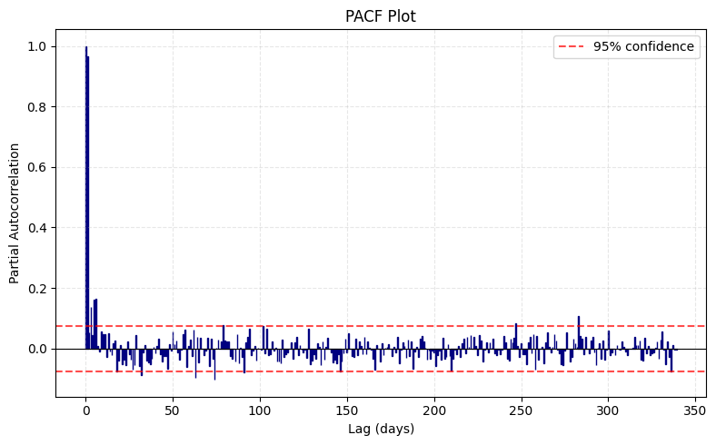
Based on the PACF plot above, given the significant spike of correlation occurs on lag 1, the data follows an AR(1) process, which suggests that the model is

The estimation of the coefficient $\phi_1$ is beyond the scope of the article. For now, it’s sufficient to understand that OLS and fast-filtering algorithms are two methods to achieve this.

Now, what if the PACF plot gradually decays instead of showing sharp peaks like the above? This suggests that the time series data instead follows a moving average (MA) process. We define an MA($q$) model to be

Note it’s similarity to an AR model, except instead of regressing on observable past values, we regress $X_t$ on past errors that we must estimate simultaneously within the model itself. We can also rewrite this function using the backshift operator into

Also, unlike the AR process, the MA process is actually stationary for all values of $\theta_1…,\theta_q$ because it’s a finite linear combination of white noise with constant mean and variance and no autocorrelation. Take a look below at the analytical expressions that shows this:

However, it’s not all sunshine and rainbows just because MA processes are guaranteed to be stationary. The important assumption for such an MA process is invertibility. This property is actually very intuitive: Because we need errors for forecasting but we can’t directly observe them, we must recover past errors from past observations. To do this, we invert the MA polynomial $\theta(B)$ to arrive at

where $\pi(B) = \theta(B)^{-1}$ is now the autoregressive operator (see above). Now that this is just an infinite-order AR process, it’s also subjected to following the stationarity assumption so the weights don’t explode. The invertibility property of the MA process simply ensures that its inversion guarantees a stationary AR process.

Checking for invertibility of an MA process is exactly the same as that for stationarity of an AR process. Given the moving average operator

we substitute $B$ with some variable $z$, equate the equation to zero, and solve for the roots. If the absolute values of these roots $|z| > 1$, then the process is invertible.

Now, MA models are fundamentally more challenging because the error terms ($\varepsilon_t,\varepsilon_{t-1},…,\varepsilon_{t-q}$) are unobservable. Therefore, unlike AR models, we need to use iterative non-linear estimation procedures like MLE, which simultaneously estimates both the coefficients and the unobserved error sequence.

For an MA($q$) model, we can identify the optimal $q$ by examining the ACF plot, which should cut off after lag $q$. If the ACF shows a gradual decay instead (such as the case in this example), this suggests that the process may follow an AR process, and therefore we should also check the PACF plot.

But what if both plots show a gradual decay with increasing lags? This is where we introduce the autoregressive moving average (ARMA) model. We say that a time series follows an ARMA($p,q$) process if it’s stationary and

As we can see from the function above, we merge the AR($p$) and MA($q$) components into a single equation. This is advantageous because it’s flexible in the sense that it captures both the autoregressive and moving average structures simultaneously.

However, there are a few challenges associated with this:

• AR components require stationarity while MA components require invertibility.
• ACF and PACF interpretation is tricky because AR and MA effects can mimic each other.
• Increased computational costs from using non-linear optimization techniques for estimation.
• Requires information criteria (AIC/BIC) to optimize bias-variance tradeoff (prevent overfitting).
• Parameter redundancy can occur when AR and MA polynomials share factors.

Now, pay close attention to the fact that the ARMA model assumes stationary data. As we’ve said many times before, this is rarely the case for real-world data. Enter the Autoregressive Integrated Moving Average (ARIMA) model.

The ARIMA model is quite literally an ARMA model that removes this stationarity restriction by incorporating an integration step. This means that it performs differencing on the data until it becomes stationary, then does everything the ARMA model already does.

We define an ARIMA($p,d,q$) to be a process the data is differenced $d$ times to become stationary, and the resulting stationary series is modeled as an ARMA($p,q$) process. Thus, we can also observe that ARIMA($p,0,q$) is exactly ARMA($p,q$). The optimal $d$ is the smallest number of differences to achieve stationarity. We can typically determine via:

• Visual inspection of a time series; if the data plot trends, difference once, and keep differencing until the trend disappears.
• Statistical tests; if ADF and KPSS tests conclude non-stationarity, difference once, and keep differencing until the tests conclude stationarity.

Before we conclude this article, I’d like to introduce one statistical test, the Ljung-Box test, which checks whether the residuals from our fitted model (AR, MA, ARMA, ARIMA) are white noise. To reiterate, we need the residuals to be white noise (i.e., i.i.d. r.v. $\sim \mathcal{N}(0,\sigma^2)$). Recall that the whole idea behind using time series models is to extract autocorrelation from the residuals. The Ljung-Box test forms the following hypotheses:

• $H_0$ : Residuals don’t exhibit autocorrelation (independently distributed).
• $H_1$ : Residuals exhibit autocorrelation.

If the test statistic rejects $H_1$, then we’re confident to say that our chosen model and its parameters have successfully captured the patterns. Otherwise, we need a better model, which means we should consider:

• Adjusting orders of $p$ and $q$,
• Opting alternative structures (e.g., ARIMA, SARIMA, ARIMAX)
• Opting entirely different model classes (e.g., exponential smoothing, GARCH)

To wrap up everything, the fundamental goal of time series models is to remove autocorrelation from the data, transferring it from the error term into the model’s structure. Each model we’ve discussed—AR, MA, ARMA, ARIMA—offers a different approach to this task. To validate our choice of model, we conduct the Ljung-Box test, where if autocorrelation remains, then we simply haven’t found the right model yet.