Time Series Talks: Looking Back

One assumption we discussed for linear regression is the independence of error terms. In that setting, we were typically dealing with cross-sectional data, where we assumed that observations don’t influence each other.

Time series data is a little special. Over time, observations are rarely ever independent. If we observe that today’s stock price is high, there’s a pretty good chance that yesterday’s price is high. In other words, values in a time series tend to be correlated with their past. We call this dependence across time autocorrelation.

As if to smoothen the transition between the two, many time series models are built on ideas that are quite similar to the typical models we use for cross-sectional data. The difference is that instead of treating correlation as a problem, we explicitly model that dependence in time series models.

***

Obviously, time series data doesn’t just comprise of two observations. So naturally, we typically ponder about how far back the dependence goes and if there are past observations that the current observation tend to be influenced by more than the rest.

Before getting our hands on the actual tools that literally answer these questions, it’s worth revising the concept of lag. Given present time $t$, then the lag-$k$ of an observation $X_t$ is $X_{t-k}$. As we’ll soon see, this idea is pervasive throughout understanding autocorrelation because it’s the whole thing that dependence of past values is built upon.

Let’s take a look at a dataset of mean daily temperatures in Jaipur, India from Kaggle.

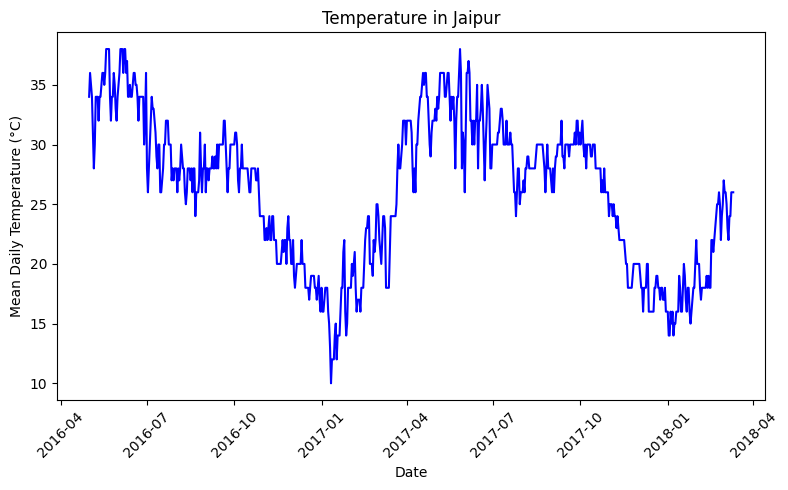
Immediately, upon first glance, the plot reveals two distinct patterns. First, the temperature follows an annual cycle. Second, within each cycle, we see a downward trend up to January, then an upward one leading to the next cycle. But of course, such conclusions are qualitative, which are useful for intuition, but not precise enough for modeling. This is where the autocorrelation function (ACF) comes in.

The ACF poses the following question: given everything we know, how strongly is $X_t$ correlated with $X_{t-k}$? In sequential data, $X_{t}$ is related to $X_{t-k}$ in this way:

Since the ACF doesn’t discriminate between direct and indirect connection, it takes into account the direct influence of $X_{t-k}$ on $X_t$, the indirect influence of $X_{t-k}$ through the sequence of lags up to $X_{t-1}$ on $X_t$, and the influence of any other chain of events that connects the two points in time.

Therefore, we define the ACF at lag $k$ to be

This is implicit in the statsmodels package in Python, and we can simply calculate the ACF by running

from statsmodels.tsa.stattools import acf
acf_values = acf(temperature, nlags=len(temperature)-1)

The graph is obtained as follows:

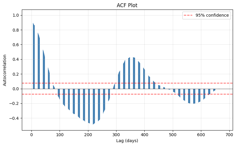
From the plot, we see a distinct cyclical pattern with a period of roughly 365 lags which corresponds to the annual seasonal cycle. We also observe a “damping” effect, where the absolute autocorrelation with past values slowly fades as the lag increases. This is expected because of inherent variability in weather patterns and potential long-term climate trends. Mathematically,

Lastly, almost all lags exceed the confidence bounds. This provides us with statistical confirmation that, indeed, there is strong seasonality, non-stationarity, and that, although out of the scope of this article, the ACF alone can’t distinguish between AR and MA components because seasonal patterns dominate.

The final observation is actually somewhat problematic. If $X_t$ correlates very strongly with $X_{t-k}$, then $X_t$ will automatically also be correlated with $X_{t-k-1}$. The ACF can’t distinguish if the correlation between $X_t$ and $X_{t-k-1}$ is direct or just because it influences $X_{t-k}$ which then influences $X_t$. This lack of resolution is exactly the problem that the partial autocorrelation function (PACF) aims to mend.

Unlike the ACF, the PACF removes the intermediate effects and so only shows us the direct correlation at each lag. To simplify the equation, we’ll define the joint intermediate lags between $X_t$ and $X_{t-k}$ as

With this, we define the PACF at lag $k$ to be

The conditioning holds the intermediate lags fixed, so any correlation explained through them is removed. For some intuition, this calculation regresses $X_t$ on the intermediate lags

then regresses $X_{t-k}$ on the intermediate lags

and then calculates the autocorrelation

In this age of technology, we can simply call the pacf function from the statsmodels package:

from statsmodels.tsa.stattools import pacf
pacf_values = pacf(temperature, nlags=int(len(temperature)/2))

And plot the results as follows:

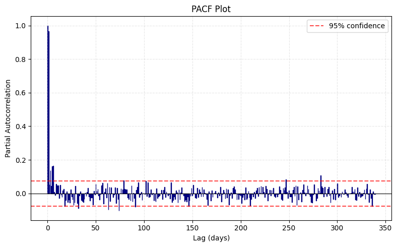
The leftmost bar will always be one because $X_t$ is always perfectly correlated with itself. The most prominent outcome of this analysis is that the mean daily temperature follows an AR(1) process given lag-1 dominates. However, we do see several other significant later lags. What do these mean?

With 339 lags and a 95% confidence level, we’d expect $339 \times0.05 \approx 17$ “significant” lags by pure chance. Our PACF analysis produced 14 of these. This suggests that apart from the massive lag-1 correlation (which is clearly real), most of these later lags are likely Type I errors. Of course, we could be wrong and these significant lags may actually mean something, but that’s the whole point of statistical tests—it’s a risk we’re willing to take!