Regression Crumbs on a Silver Platter

There was a time when I used to apply linear regression to some data and if the resulting metrics ($R^2$, RMSE, MAE, etc.) were unsatisfactory, I simply concluded that the regression wasn’t a good fit and I should probably instead look at other models like gradient boosting or neural networks. If you don’t think this was a problem, see it in this way: a baker judges whether a cake is baked properly just by looking at the clock, without ever inserting a toothpick to check inside the cake.

The issue is that we tend to only use metrics to determine the fit of a model to data. This is problematic because linear regression, like many models, work under assumptions—assumptions that may be silently violated under the guise of a high $R^2$ value. And if the metrics show poor results, it gives us no information why this is so.

From what we’ve just discussed, it’s clear that we need to ascertain the appropriateness of using some model, in this case linear regression, for a specific application. This is where residual analysis comes into the picture.

Residuals

We’ll look at the simple case of a linear regression model with one predictor:

where the true error $\varepsilon_i$ is estimated by the residual $e_i$, which is the difference between the observed value $Y_i$ and fitted value $\hat{Y}_i$:

The assumption of the regression model is that the error term $\varepsilon_i$ is an independent normal r.v. with mean zero and constant variance $\sigma^2$. The basic idea behind residual analysis is to examine whether $e_i$ reflects the properties assumed for $\varepsilon_i$ (meaning the model is appropriate if so).

Just like how $\varepsilon_i$ is an r.v., $e_i$ also is. We’ll therefore also lay out the mean and variance of the residual in the simple linear regression context as follows:

• $\bar{e} = \frac{\sum e_i}{n} = 0$
• $s^2 = \frac{\sum(e_i – \bar{e})^2}{n-2} = \frac{SSE}{n-2} = MSE$

With that out of the way, we can move on to define six important departures from the simple linear regression model with normal errors:

1. Non-linearity of regression function
2. Heteroskedasticity
3. Presence of outliers
4. Non-independence of error terms
5. Non-normality of error terms
6. Omission of important predictor variables

As we’ll soon see, residual analysis diagnoses these departures! Additionally, we’ll also consider one or several mediations to realign the data back to the proper assumptions.

Non-linearity of Regression Function

Let’s take the example of regressing the unit price of a certain toy to the total revenue for an imaginary toy company ABC. The regression is presented in the scatter and residual plots below.

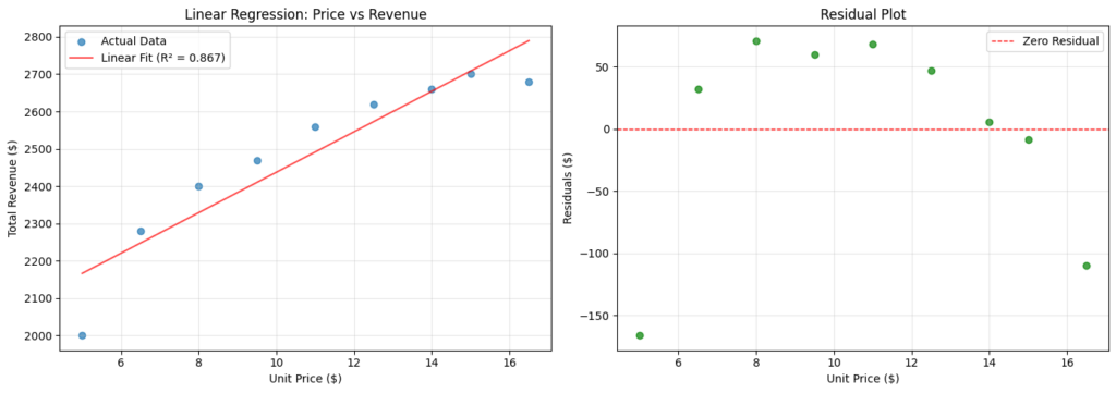
The preference for using a residual plot to visualize linearity (or lack thereof) is in how much more clearly it shows the deviations of each residual from zero. Often, it’s sufficient to conclude linearity from simply visualizing the residual plot.

To mitigate this, we can apply a transformation on $X$ (unit price). It so happens that $X\prime = \sqrt{X}$may improve linearity when regressed to the total revenue. We avoid transforming $Y$ especially if the error terms are reasonably close to being normally distributed and have approximately constant variance as this may change the distribution and lead to substantially differing error term variances.

Heteroskedasticity

Heteroskedasticity refers to a property of a dataset whose error variance is not constant. This is undesirable given linear regression assumes an error term with constant variance. Consider a different example: regressing income to expenditure on food. The residual and absolute residual plots are presented below.

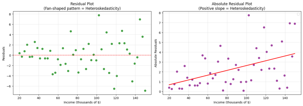
The data is said to be heteroskedastic if the residual plot exhibits a fan-shaped pattern (left). In addition to visualization, there exists several tests we can conduct to check for heteroskedasticity:

• Rank correlation test (e.g., Spearman) on the absolute residuals. In our example, the Spearman correlation is 0.469 ($p$-val: 0.0006; reject homoskedasticity)
• Brown-Forsythe test on the residuals. The intuition is to split the data into two groups (small $X$ vs large $X$) and compare each group’s absolute median from the group median. Here, the test statistic is 8.67 ($p$-val: 0.0050; reject homoskedasticity)
• Breusch-Pagan test on the squared residuals. BP aims to regress $e_i$ to $X_i$, and tests whether $X_i$ explains $e_i$ (implying heteroskedasticity). The test statistics $LM$ and $F$ for our dataset is 9.93 ($p$-val: 0.0016; reject homoskedasticity) and 11.9 ($p$-val: 0.0012; reject homoskedasticity) respectively.

Transformations are our best friend to “fix” non-constancy of error variance. Specifically, we typically apply a transformation on $Y$. In this case, the transformation $Y\prime = \log_{10}Y$ seems to have brought the residuals closer to homoskedasticity.

Presence of Outliers

Although residual outliers can be identified using residual plots, plotting semi-studentized residuals is golden because it lets us visualize how many standard deviations from zero the outliers are.

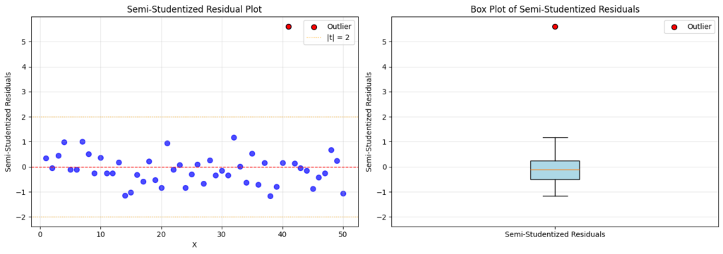
The test for outlying or influential variables is pretty straightforward. We simply rerun the regression without the outlier (using $n-1$ variables) on the semi-studentized residual data and calculate the probability of seeing the outlier in $n$ observations. Our $t$-statistic for this is 10.1 ($p$-val << 0.05; reject data point is not an outlier), meaning it’s indeed very likely an outlier.

Non-independence of Error Terms

Recall that one assumption of linear regression is independent error terms. This assumption is often violated in time-series data because of autocorrelation, making the residuals trend or cycle periodically. We consider the plots for some cyclical (and therefore non-independent error terms) time-series data below.

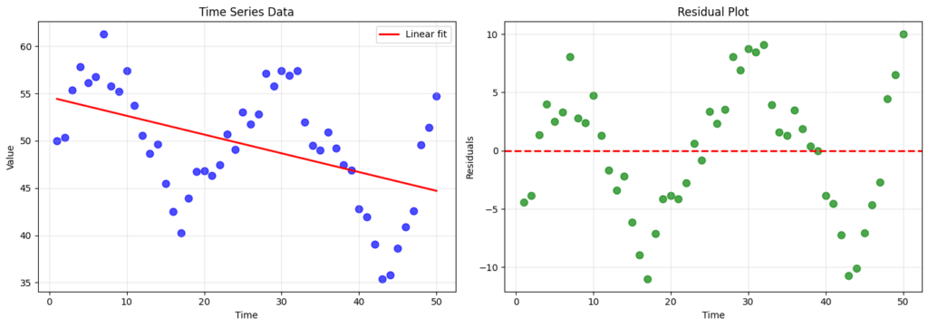
It’s painfully obvious how autocorrelated the residuals are. However, sometimes, the relationship may not be obvious and so we may want to perform a Wald-Wolfowitz runs test. Its intuition is actually very elegant: random data should alternate unpredictably, while patterned data will show too much (too many runs) or too little (too few runs) alternation. For our dataset, the test statistic is -5.11 ($p$-val << 0.05; reject independence).

A nice amelioration of non-independent error terms is by instead regressing on the first differences

where $\Delta Y_t = Y_t – Y_{t-1}$ and $\Delta X_t = X_t – X_{t-1}$ given the original model

The nuances of this transformation is actually very important and common in the field of time-series analysis, which is out of the scope of this article and so won’t be discussed further.

Non-normality of Error Terms

Various plots can be visualized to examine the normality of error terms. Among which are box plots, histograms, and normal probability plots. In normal probability plots, or Q-Q plots, each residual is plotted against its expected value under normality. A plot that is nearly linear suggests agreement with normality, whereas those that largely deviate from linearity suggests a non-normal distribution.

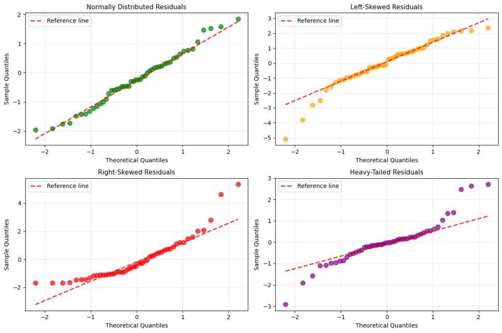
Employing goodness of fit tests, such as the chi-square, Kolmogorov-Smirnov, or Shapiro-Wilk test, on residual data is a common method for testing normality of error terms. For instance, using Shapiro-Wilk, the $p$-value is 0.672 (failure to reject normality) for the top-left plot, and 0.014 (reject normality) for the top-right plot.

Unlike the other model departures, the analysis for non-normality of error terms is more difficult because it’s affected by the remediation for other departures. However, non-normality and non-constancy of error terms often occur simultaneously in a dataset. As a result, by applying the transformation $Y\prime = \log_{10}Y$ mentioned previously, we actually also enforced the distribution to be more approximately normal. The only issue is that this may also cause non-linearity, which therefore requires us to also simultaneously transform $X$ to maintain linearity.

Omission of Important Predictor Variables

This last model departure is the simplest of all, which simply explains that all variables that contribute to the model’s appropriateness for the dataset must be included. Consider a scenario where a company employs two teams to manufacture a product, one with advanced machinery and one as manual labour. It’s important that we include both teams as predictor variables for downstream regression against the total time taken to produce the goods. Obviously, considering only the efficient team skews the model upwards, while considering the latter skews the model downwards.

Final Notes

Notice that the remedial measures we took were all such that it modified the data and not the model. This is intentional, as I want to focus on specifically showing how we can mitigate model departures to use, specifically, simple linear regression (technically also multiple linear regression for the omission of important predictor variables).