To Squish Data and Not Break It

I always knew Principal Component Analysis (PCA) as a dimensionality reduction technique. Way too many features? PCA. Need to visualize clustering? PCA. Exploratory data analysis? PCA. It’s definitely one of my go-to analysis back then, but not because of its usefulness—it was one of the few tools I knew existed, so might as well, I thought. When I ventured deeper into statistics, this was one of the first few things I mastered because it was a technique I used so often.

Like I mentioned, PCA is a powerful tool for dimensionality reduction, feature engineering, and data visualization. Essentially, it linearly transforms data inputs into a new coordinate system with new axes called principal components. I can’t wait to delve into the how’s of PCA, but it’s definitely wise to lay out some very important terms to aid the explanation.

Orthogonality

Orthogonality is a generalization of perpendicularity. In plane geometry, two lines that are perpendicular intersect each other at 90°. Mathematically, in 2D and 3D Euclidean space, we say that the dot product of two perpendicular vectors $\mathbf{u}$ and $\mathbf{v}$ satisfies

Orthogonality simply extends this notion to non-physical spaces (e.g., space of functions, abstract vectors) and situations where the concept of angles may not be obvious but the algebraic relationship generalizes the 90° idea. It’s defined by an inner product (a generalization of the dot product) where $u$ and $v$ are orthogonal if

This is equivalent to $\mathbf{u} \cdot \mathbf{v} = 0$ for perpendicular vectors, but now $u$ and $v$ could be functions, matrices, abstract vectors, etc.

The Eigen-equation

Vectors can undergo different types of linear transformations to stretch and rotate, often changing their magnitude (length) and direction. But, for a given transformation, there are special vectors that, when transformed, do not change direction, only magnitude. These special vectors are called eigenvectors. They only get stretched or squashed, and the factor by which they are stretched or squashed is called the eigenvalue.

Let’s represent some transformation as a square matrix $A$. Applying this transformation to the eigenvector $\mathbf{v}$ by multiplying them is equivalent to scaling $\mathbf{v}$ by a factor of $\lambda$:

We call this equation the eigen-equation.

The How of PCA

The most intuitive explanation of PCA comes alongside an example. Suppose we have a dataset for the heights and weights of four students as shown in the table below.

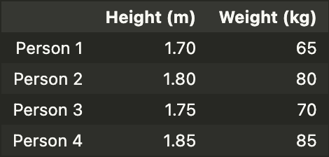
The first step is to standardize the data for each of the features:

data_z = (data - data.mean()) / data.std()

We do this to allow the variance of each feature to be at the same degree of magnitude as each other. This is very crucial because, as will be explained in greater depth later, PCA works by finding directions of maximum variance. Without standardizing, we can see that the variance of the weight is about 17,000 times that of the height:

• $\text{Var}(h) = 0.00313$ m$^2$
• $\text{Var}(w) = 54.7$ kg$^2$

This results in a scale bias, where the principal components become dominated by variables with the largest absolute variances simply because they’re measured in larger units and not because they’re statistically more important. Standardizing the dataset eliminates this bias.

The next step is to calculate the covariance matrix of the standardized dataset:

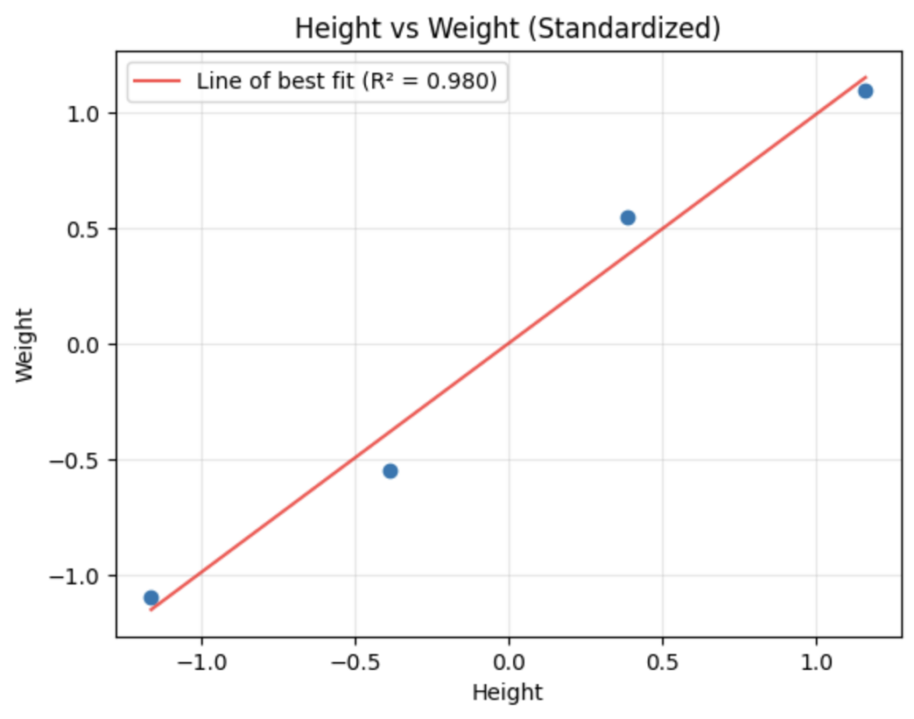
cm = data_z.cov()

To understand why we need the covariance of the dataset for PCA, we consider explaining the intuition form the perspective of PCA as an optimization problem. As mentioned, the goal of PCA is to find directions of maximum variance. To do this, in the regressive sense, it has to minimize the sum of squared deviations (i.e., find the line of best fit). The visualization is provided as follows:

Mathematically, we begin with a dataset of $n=4$ points, each a standardized vector $\mathbf{x}_i$. Our goal is to find a unit vector $\mathbf{v}$ (i.e., the direction of the first principal component) which maximizes the variance of the projected data. The projection of a data point $\mathbf{x}_i$ onto $\mathbf{v}$ is just the inner product

and the variance of these projections across all points is

With a clever manipulation using matrix operations,

where $\mathbf{x}_i \mathbf{x}_i^{\intercal}$ is an outer product. Therefore,

I know it took a while to get here, but notice that the expression in the parentheses is precisely the covariance matrix $C$ of the standardized dataset! Things get even cooler when we realize that the optimization problem is now to maximize $\mathbf{v}^{\intercal} C \; \mathbf{v}$ given the vector must be unit length (constraint):

Using Lagrange multipliers, we want to maximize

Taking the derivatives with respect to $\mathbf{v}$ and setting it to zero,

which finally simplifies back to our eigen-equation

By understanding the above, we have proven that the directions we want (the principal components) are mathematically forced to be the eigenvectors of the covariance matrix $C$.

If we were to compute the eigenvectors and eigenvalues manually, we would calculate them via the determinants $\det(C – \lambda I) = 0$. Realistically, in code, packages use numerical algorithms like SVDs for numerical stability:

from sklearn.decomposition import PCA
pca = PCA(n_components=2)
pca.fit(cm)

Up to this step, we’ve actually finished the run. All that’s left to do is some analysis of the transformed data. Typically, we’re interested in the eigenvalues (i.e., explained variance ratio):

and also the eigenvectors:

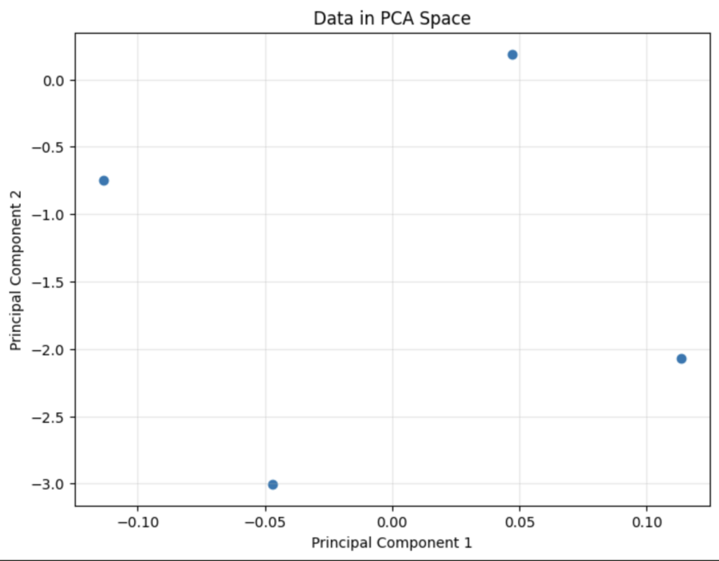
Given the eigenvalues, we observe that the data is actually 1-dimensional, where all the variance in the data is explained by just one principal component. Looking at the loadings of each component in the eigenvector (PC1), we also learn that all the variation can be explained by a “slenderness” axis. Finally, since the transformed data is 2-dimensional, we can visually plot the newly transformed data with the principal components as the axes.

Solution to Multicollinearity

I just wanted to also point out how PCA could be a method to solve multicollinearity in datasets, which is an issue where predictor variables are highly correlated. By definition, principal components are orthogonal, meaning the transformed axes have zero correlation. In other words, by using the principal components as the predictor variables, multicollinearity is completely eliminated. However, we lose some interpretability by doing this as principal components are combinations of original variables.

Today, there exist so many different variants of PCA designed to address specific limitations or adapt to different data types. For instance, Kernel PCA uses kernel trick to find non-linear patterns and Robust PCA uses robust estimates of covariance to reduce sensitivity to outliers. Perhaps I shall come back to this topic again and cover them in the future.