Everything is Normal

The normal distribution is one of statistics’ most precious models of reality. It’s analytically tractable, computationally simple, and provides a universal language for uncertainty. As such, it definitely deserves an in-depth exploration of its characteristics, properties, and significance. And then, we’ll explode in, Game of Thrones style, to ruin the perfect rainbow world of normality by introducing the real world we live in.

The normal (Gaussian) distribution is the most famous continuous distribution with a bell-shaped p.d.f. $\varphi$, defined by only two parameters: mean $\mu$ and standard deviation $\sigma$. Given a normal r.v. $X \sim \mathcal{N}(\mu, \sigma^2)$,

Having two descriptive statistics, $\mu$ and $\sigma$, be the parameters of the model makes the Gaussian a generalist model in data analysis. In other words, given only the mean and spread of a phenomenon that results from many independent random contributions, the normal is the natural, most conservative model for its behavior.

Another beautiful mathematical property of the normal distribution is that normal r.v.s are closed under addition. Essentially, the linear combination of normal variables are normal. This is powerful because it’s become the foundation upon which various statistical models are built. Linear regression is a prime example of this.

Given the linear regression model

where $\varepsilon \sim \mathcal{N}(0,\sigma^2)$. Under the closure under addition property, we are certain that $Y$ also follows a normal distribution $Y \sim \mathcal{N}(\beta_0 + \beta_1 X, \sigma^2)$. Thanks to this, estimating $Y$ can be done alongside reporting a confidence interval as a means of uncertainty quantification. The only issue is that the true variance $\sigma^2$ is often not known, and hence must be estimated from the data, meaning we actually use the $t$-distribution instead (and not the normal) for small sample confidence intervals.

Interestingly, the normal distribution isn’t even its simplest form. Enter the standard normal r.v. $Z$, given by

I call this the “final form” of the normal distribution because of how simplified it’s become. With $\mu=0$ and $\sigma^2=1$, this is quite literally pure randomness; Gaussian noise.

If we plot the standard normal distribution as below, a cool characteristic, called the empirical rule, can be visualized.

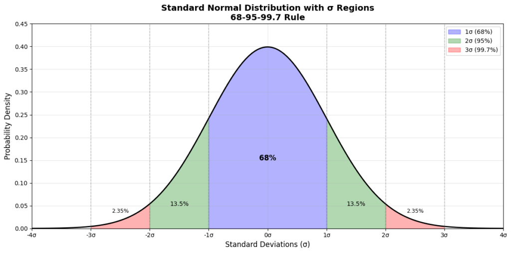
What we see is that:

• ~68% of observed data falls within $1\sigma$
• ~95% of observed data falls within $2\sigma$
• ~99.7% of observed data falls within $3\sigma$

This builds the basis of the $Z$-test statistic. Since we already understand that the $Z$-score is literally pure randomness, the interpretability of this test becomes obvious—regardless of data origin, assuming it follows a normal distribution, we interpret the rule as that there is a ~32%, ~5%, and ~0.3% chance of the observed data falling outside $1\sigma$, $2\sigma$, and $3\sigma$ by pure chance. When we set the significance level (typically at $2\sigma$, corresponding to ~5%) and the observed data falls outside this boundary ($p$-value < 5%), we consider that the data may not have actually come out of the “pure randomness” distribution, and therefore reject the null hypothesis that the observation is just a product of random chance.

But there are still some holes left in our explanation. For instance, how dare we model the error term in linear regression as a normal distribution? This perfectly transitions us to another elegant vindication of the normal distribution: the central limit theorem (CLT).

CLT states that the sum (or average) of a large number of i.i.d. r.v.s will be approximately normal, regardless of the underlying distribution of the variable. Mathematically, as $n \rightarrow \infty$,

The error term $\varepsilon$ in the linear regression (or other) model is basically an aggregation of thousands of tiny, independent, ignored effects that aren’t in the model. This is precisely what the CLT defines to be approximately normal. In other words, we model $\varepsilon$ as normal because theoretically, the net effect of everything we forgot to measure tends to be normal.

Like I mentioned, unfortunately, reality rarely reads a textbook. Simply slapping on “normally distributed” labels on everything is extremely naive.

First, in a normal distribution, extreme events many standard deviations away from the mean is virtually impossible; they are theoretically events that should only happen once in a million years. However, the world has fat tails, that is, we see rare events (e.g., market crashes, wars, pandemics) occur much more often than what a normal distribution suggests. Secondly, regressions relying on normality assume i.i.d. error terms. In reality, errors cluster, correlate, and carry memory (i.e., they’re not independent). Thirdly, the normal distribution is symmetric and infinite, but the real world is skewed and bounded. For instance, dramatic crashes in the stock market occur more frequently than dramatic rallies, and prices, incomes, and wait times are among variables that cannot go below zero (i.e., bounded). Lastly, the ugly side of the CLT is that it takes its own sweet time before the effects kick in, meaning the “large” could mean hundreds, thousands, or millions of samples, making the assumption of normality but a pipe dream in fields where data is scarce.

I’m not saying that normality is bad, though. If you’ve already made sure to diagnose that the assumption of normality is valid, then go work your magic.