Time Series Talks: Consistency is King

One of the most important assumptions for statistical models to work is the notion of consistency. This means that statisticians often drool with excitement when they find out that their data has approximately stable statistical properties, because they can finally unlock the cabinet of unused dusty models.

In time series analysis (and several other disciplines), this consistency is coined stationarity.

***

Stationarity is often defined in two ways: strictly and weakly. Strict stationarity requires that the joint distribution of a set of values be the same for all time points. Mathematically, given the set of values at time $t$,

strict stationarity enforces that

for all positive integers $k$ and shifts $h$. Given that the probability distribution is constant, this implies that the mean and covariance are also constant. Unfortunately, achieving this version of stationarity is often too restrictive for most applications. Therefore, we’ll also introduce a milder version which only restricts the first two moments of the series.

The weak stationarity is a condition where only the mean and covariance of a series are constants. Given the leniency of this property, we typically understand that weak stationarity is implied if a series is said to exhibit stationarity.

In other words, if we let $k=1$ and consider any two time points $s$ and $t$,

• $\mu_{s} = \mu_{t}$
• $\gamma(s,t) = \gamma(s+h,t+h)$

If we get our hands on some time series data, of course we may want to consider whether it’s stationary so we know what models we can use. The easiest way to do this is by simply visualizing the data.

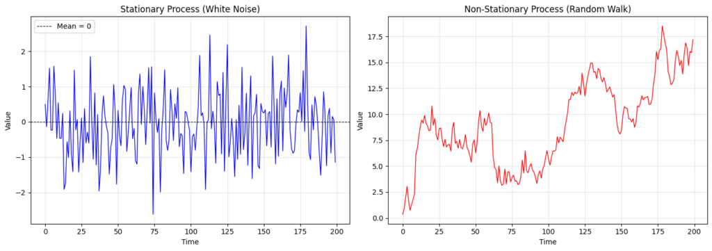
The most obvious sign that a random walk is not stationary is by observing how its mean isn’t constant. White noise, on the other hand, is widely known to be a stationary process because it comes from a standard normal distribution. However, the data we typically work with rarely ever come from an elegant distribution like the two above. In this case, we may consider conducting an Augmented Dickey-Fuller (ADF) or, try to read it out loud, Kwiatkowski-Phillips-Schmidt-Shin (KPSS) test.

from statsmodels.tsa.stattools import adfuller, kpss

sig = 0.05

# ADF Test
adf_res = adfuller(data, regression='c', autolag='AIC')
if adf_res[1] < sig:
    print(f"Series is STATIONARY (p: {adf_res[1]})")
else:
    print(f"Series is NON-STATIONARY (p: {adf_res[1]})")

# KPSS Test
kpss_res = kpss(data, regression='c', nlags='auto')
if kpss_res[1] < sig:
    print(f"Series is NON-STATIONARY (p: {kpss_res[1]})")
else:
    print(f"Series is STATIONARY (p: {kpss_res[1]})")

The intuition is that ADF tests whether past values predict the current value too strongly (via determination of a unit root) while KPSS tests if the variance grows over time. Typically, the best practice is to use both and see if the tests agree with each other. If they conflict, the series might be borderline (e.g., trend-stationary). In our case, as expected, there is overwhelming evidence ($\alpha=0.05$) that the white noise is stationary ($p_{ADF}<<\alpha$ and $p_{KPSS}=0.10$) and random walk isn’t ($p_{ADF} = 0.37$ and $p_{KPSS} = 0.010$). Note that the null hypotheses for both tests are opposites.

Cool, now we know which process is stationary and which isn’t. Now, want to work with the stationary counterpart of the random walk. How can we achieve this? The most common method is differencing. For instance, take a look at the following plot for the adjusted close price data of SPY from 2020 to 2024.

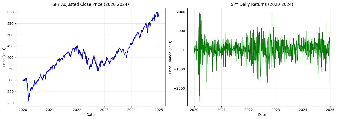
It’s clear by visualization that the price path (left plot) is non-stationary. The ADF and KPSS test-statistics are -0.109 ($p=0.948$; reject stationarity) and 4.43 ($p=0.010$; reject stationarity), further supporting our observation. We now calculate the price difference,

to get the price change path (right plot), which already looks stationary. The ADF and KPS test statistics are -11.1 ($p<<\alpha$; reject non-stationarity) and 0.123 ($p=0.100$; reject non-stationarity), which also supports this.

Note that this price change is not the same as returns in finance, which is

Returns also exhibit stationarity. Since we’re on this topic, I’ll leave it up to you to plot and calculate the test statistics to conclude yourself.