Making Waves with Fourier

In the context of time series analysis, as statisticians, we’re more than comfortable with thinking about data in the time domain. Here, we have values which evolve across time, and the questions we’re interested in often follow this perspective: Is the series trending? Is it noisy? Is today’s data dependent on yesterday’s?

This view is extremely useful but also has its limits. Real data is noisy. Sometimes, what looks like chaotic noise is actually the result of multiple cyclical patterns layered on top of each other. When these signals combine, the resulting time-series can look so tangled that the underlying patterns become nearly impossible to see.

This is why we must also love the frequency domain. Solving the problem I’ve just laid out is the very foundation for why the frequency domain is powerful. And to bridge the two perspectives, we’ll discuss a technique called the Fourier transform.

***

Let’s talk about some important concepts that will eventually unite to form the basis of Fourier transform.

Recall that the inner product of two functions $f(t)$ and $g(t)$, $\langle f,g \rangle$, is given by

where $\bar{g(x)}$ is the complex conjugate of $g(x)$. This inner product measures how much $f$ resembles $g$, and the value is large if they move together (and small if unrelated).

Another important topic is orthogonality, which is a property in which the inner product of two functions equal zero. Recall that this is equivalent to how the dot product of two basis vectors equal zero. Consider the following plot for $f(t) = \sin(t) \sin(2t)$ for $0 \le t \le 2\pi$.

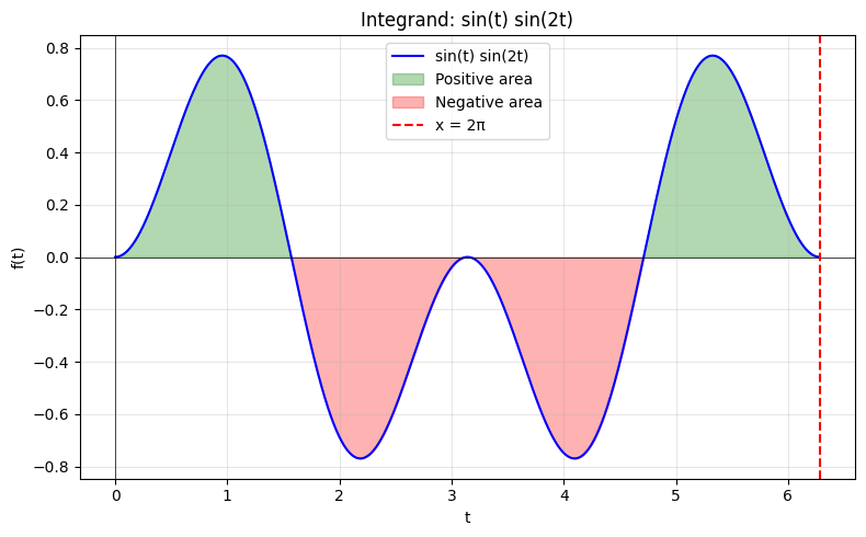
Calculating the inner product between two functions $h(t) = \sin(t)$ and $g(t) = \sin(2t)$,

as we can see from summing the area under the curve in the plot above. We can confirm this analytically, but we won’t. More importantly, this means that $h$ and $g$ are orthogonal functions. As it turns out, this orthogonality in fact holds for any two different frequencies—sine (and cosine) waves of different frequencies are perpendicular in function space. We can also confirm this analytically, but again, we won’t.

How do these relate to Fourier transform, the bridge between time and frequency domain? Let’s assume the following multilayered signal:

where $\omega_1$ and $\omega_2$ are frequencies inside the signal. To measure how much of $\omega_2$ lives in this signal, the natural approach given what we’ve discussed is to take the inner product with a pure tone at that frequency

By orthogonality, $\sin(\omega_1 t)$ contributes nothing, while $\sin(\omega_2 t)$ paired with itself yields some positive value. In this case, our pure tone example perfectly captures the frequency of interest. Now consider a different signal

The same inner product with $\sin(\omega_2)$ returns zero because $\cos(\omega_2 t)$ and $\sin(\omega_2 t)$ are orthogonal. In other words, although the frequency $\omega_2$ exists, our measurement completely misses it because the cosine component slips through unseen. To reliably capture any wave at frequency $\omega_2$, regardless of its wave, we need both orthogonal test waves to catch the cosine and sine components.

There’s technically no issue with this because we’ll properly capture $\omega_2$ by taking the inner product $\langle h(t), \sin(\omega_2 t) + \cos(\omega_2 t)\rangle$. The orange flag with this computation is that it gets annoying and messy to always have to account for two values for every frequency.

The elegant solution to this is the Euler’s formula

As you can see, Euler’s formula unifies the two components into a single complex exponential function. Now, the inner product $\langle h(t), e^{i\omega_2 t} \rangle$ returns a complex number whose real part is the cosine component and imaginary part the sine component.

Let’s write out the integral equation for this inner product for any signal $f(t)$ and frequency $\omega$:

So far, we’ve been using periodic signals like $\sin(\omega t)$ and $\cos(\omega t)$, which allows us to capture all that information inside a single period $2\pi$ (because their patterns repeat identically outside the window). However, real-world data like stock prices and brain waves are rarely periodic—events happen once and never repeat exactly. If we restrict ourselves to a fixed period, we risk missing whatever occurs outside the boundary. Hence, we must account for the entire span of the series, and therefore extend the integral to infinite bounds:

where the exponent is appended with a negative purely for convention to make the inverse of the function simpler. This, ladies and gentlemen, is also known as the Fourier transform.

If we’re done working on the data in the frequency domain, we can also transform it back to the time domain using the inverse Fourier transform

where $2\pi$ is a normalizing constant that exists to ensure that applying the forward transform followed by the inverse returns the original function exactly.

Actually, the continuous Fourier transform is a mathematical ideal. In reality, data is discrete. Next time, we’ll discuss two of its popular variants: discrete Fourier transform and fast Fourier transform, where we can truly bridge the gap between theory and application on real data.